Difference between revisions of "Se170063"
| (52 intermediate revisions by 2 users not shown) | |||
| Line 2: | Line 2: | ||
=Sample Description= | =Sample Description= | ||
| − | The sample was placed in an aluminum cylinder that was to be irradiated. The target components consisted of a nickel foil on the front of the cylinder with 2 pure selenium pellets under the foil, but still outside the cylinder. Inside the target there was burnt sagebrush ash, which was | + | The sample was placed in an aluminum cylinder that was to be irradiated. The target components consisted of a nickel foil on the front of the cylinder with 2 pure selenium pellets under the foil, but still outside the cylinder. Inside the target there was burnt sagebrush ash, which was place in an oven, and selenium. Below are the masses of the components |
Nickel Foil: 0.2783g | Nickel Foil: 0.2783g | ||
| Line 18: | Line 18: | ||
The Calibration for Detector A was done on the morning of 5/23/17 with the MPA software using the thorium rods (as the calibration was fairly close already) and the correction values were found to be Det A Intercept = -12.208800 slope =1.021270 | The Calibration for Detector A was done on the morning of 5/23/17 with the MPA software using the thorium rods (as the calibration was fairly close already) and the correction values were found to be Det A Intercept = -12.208800 slope =1.021270 | ||
| − | + | Se170063 Thin Window Analysis | |
=Efficiency= | =Efficiency= | ||
| Line 24: | Line 24: | ||
=Nickel Information= | =Nickel Information= | ||
| − | |||
| − | [[ | + | [[Se170063 Nickel Investigation]] |
| − | + | =Activity and Half Life= | |
| + | [[Se170063 Activity And Half Life]] | ||
| − | + | The method that has given the most acceptable results is given in [[Se170063 Thin Window Analysis]] | |
| − | + | Compare Rates between Two pure SE samples Irradiated at same time and measured using same detector with samples at the same location | |
| − | + | [[Se_5-25-17-RateCompare_OuterSe]] | |
| − | + | =Alternative Method= | |
| − | + | [[Se170063 Activity and HL Alternate]] | |
| − | + | =Corrected Alternative method= | |
| − | + | The files used for this analysis are in the directory /data/IAC/Se/May2017/5_25_17/Se_Activity_SysOffset_Mix | |
| − | |||
| − | |||
| − | |||
| − | |||
| − | |||
| − | + | To begin, I have corrected the mixture to have a factor of 0.62, which is the mystery factor throwing of all of these analyses. The histogram is also weighted by the mass. The weight added to the histogram is | |
| + | <math> h1 -> Fill(evt.Chan,\frac{1}{0.0523*0.62}) </math> | ||
| − | Below is the | + | So the true number of counts has indeed been weighted here. Now I want to try to test every different method that was suggested. So first I am going to weight the mixture by the mystery factor of 0.62, and leave my Gaussian fits as wide as they were previously. The gaussians will probably be made more compact if the mystery factor does not alleviate the problem. The first step is to find the number of counts within the window of interest. Below is the process I used to determine the number of counts and the error associated with it. First begin by plotting the histogram using the ROOT program Eff.C, which is shown below. |
| − | [[File:170063 | + | [[File:170063 Spec Weighted.png|200px]] |
| + | Now take the integral given in the stats box and subtract the background to get the number of counts. Here the number of counts would be | ||
| − | + | <math> 927800 - 47670 = 880130 Counts </math> | |
| − | + | Now I can convert this error into an activity by dividing by the time, which is 300 seconds in this case. After that take the natural log of the quotient. | |
| − | <math> \ | + | <math> \ln{\frac{880130}{300}} = 7.984042428 </math> |
| + | Now to find the error we can notice that the standard deviation here is 0.6238. The procedure is to expand the window by one or two standard deviations and find the difference in the number of counts in the original window. Due to the binning here I have decided to expand the window by 1 channel on each side, which is roughly 2 standard deviations. A picture is given below. | ||
| − | + | [[File:170063 Spec ExpandedWindow.png|200px]] | |
| − | + | Now we do a similar method to find the number of counts within this window. | |
| + | <math> 1017000 - 46810 = 970190 Counts </math> | ||
| − | + | Now take the difference between the original window's number of counts and the expanded window's number of counts. | |
| − | = | + | <math> 970190 - 880130 = 90060 Counts </math> |
| − | |||
| − | + | Now to propagate this error we must divide this number by the original number of counts. | |
| − | + | <math> \frac{90060}{880130} = 0.1023257928 </math> | |
| − | + | This method was repeated for the next set of runs that make the data file. The numbers are in a table below. | |
| − | + | {| border="3" cellpadding="5" cellspacing="0" | |
| + | || || 0 <t< 300 sec || 730 < t < 1020 sec || 1480 < t < 1775 || 2250 < t < 2550 sec || 3050 < t < 3300 sec || 3775 < t < 4050 sec || 4480 < t < 4770 sec | ||
| + | |- | ||
| + | ||Original Window Counts || 880200 || 716200 ||617100 || 545800 ||394100 || 362000 || 346300 | ||
| + | |- | ||
| + | || Original Window Background (Integrated) || 381379 || 267608 || 215260 || 189665 || 143921 || 137541 || 128197 | ||
| + | |- | ||
| + | ||Original Window Difference || 498821 || 448592 || 401850 || 356135|| 250179 || 224459 || 218103 | ||
| + | |- | ||
| + | ||Expanded Window Counts || 970900 || 782600 || 671300 || 593100 || 426700 ||395400 ||378100 | ||
| + | |- | ||
| + | ||Expanded Window Background || 468138 || 333633 || 269025 || 236476 || 173353 ||170089 || 159644 | ||
| + | |- | ||
| + | ||Expanded Window Difference || 502762 || 448967 || 402275 || 356624 ||253347 || 225311 || 218456 | ||
| + | |- | ||
| + | ||Error in counts || 3941 || 375 || 425 || 489 || 3168 || 852 || 353 || | ||
| + | |- | ||
| + | ||.dat file entry || 7.416220118 +/- 0.0079006297 || 7.343988145 +/- 0.0008359489264 || 7.216858801 +/- 0.0010576086 || 7.079282677 +/- 0.0013730748 || 6.908471023 +/- 0.012662933 || 6.704677244 +/- 0.0037957934 || 6.622841784 +/- 0.0016185014 | ||
| + | |- | ||
| + | |} | ||
| − | + | Below is the graph that contains the information about the initial activity and the half life | |
| − | |||
| − | |||
| − | + | [[File:170063 WindowExpand WideGauss HLPlot.png|200px]] | |
| − | + | The slope of the line is -0.00019198 +/- 4.13511e^-7, which gives a half life of | |
| − | <math> \ | + | <math> t_{\frac{1}{2}} = \frac{\ln{2}}{\lambda}\rightarrow 60.18 minutes </math> |
| − | + | While the error is | |
| − | + | <math> \sigma_{t_{\frac{1}{2}}} = \frac{\ln{2}*\sigma_{\lambda}}{\lambda^2} \rightarrow 0.13 minutes </math> | |
| − | |||
| + | The constant value given by the plot is 7.4918 +/- 0.000927611, which gives an initial activity of | ||
| − | + | <math> A_0 = e^{7.4918} = 1793.28 Hz </math> | |
| − | + | and an error of | |
| − | <math> | + | <math> e^{7.4918}*\sigma_{A} = 1.66 Hz </math> |
| − | + | Now correcting for the efficiency we have | |
| − | <math> | + | <math> A_0^' = \frac{A_0}{\epsilon} = \frac{1793.28}{0.007} = 256182.8571 Hz </math> |
| − | + | While the error is | |
| − | + | <math> \sigma_{A_0^'} = \frac{A_0}{\epsilon^2}*\sigma_{\epsilon} = 402.57 Hz </math> | |
| − | + | Below are the related pages for this sample using this method of window expansion: | |
| − | [[ | + | [[Se170063 Nickel Foil Wide Gauss Window Expansion]] |
| − | |||
| − | + | [[Se170063 Pure Se Wide Gauss Window Expansion]] | |
| − | |||
| − | |||
| − | |||
| − | |||
=Runlist= | =Runlist= | ||
Latest revision as of 17:54, 9 November 2017
PAA_Selenium/Soil_Experiments#Selenium_Sample_Analysis
Sample Description
The sample was placed in an aluminum cylinder that was to be irradiated. The target components consisted of a nickel foil on the front of the cylinder with 2 pure selenium pellets under the foil, but still outside the cylinder. Inside the target there was burnt sagebrush ash, which was place in an oven, and selenium. Below are the masses of the components
Nickel Foil: 0.2783g
Outer Se Pellets: 0.0971g
Sage Ash: 0.5111g
Inner Se Pellets: 0.0523g
Energy
The Calibration for Detector A was done on the morning of 5/23/17 with the MPA software using the thorium rods (as the calibration was fairly close already) and the correction values were found to be Det A Intercept = -12.208800 slope =1.021270
Se170063 Thin Window Analysis
Efficiency
Nickel Information
Activity and Half Life
Se170063 Activity And Half Life
The method that has given the most acceptable results is given in Se170063 Thin Window Analysis
Compare Rates between Two pure SE samples Irradiated at same time and measured using same detector with samples at the same location
Se_5-25-17-RateCompare_OuterSe
Alternative Method
Se170063 Activity and HL Alternate
Corrected Alternative method
The files used for this analysis are in the directory /data/IAC/Se/May2017/5_25_17/Se_Activity_SysOffset_Mix
To begin, I have corrected the mixture to have a factor of 0.62, which is the mystery factor throwing of all of these analyses. The histogram is also weighted by the mass. The weight added to the histogram is
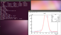
So the true number of counts has indeed been weighted here. Now I want to try to test every different method that was suggested. So first I am going to weight the mixture by the mystery factor of 0.62, and leave my Gaussian fits as wide as they were previously. The gaussians will probably be made more compact if the mystery factor does not alleviate the problem. The first step is to find the number of counts within the window of interest. Below is the process I used to determine the number of counts and the error associated with it. First begin by plotting the histogram using the ROOT program Eff.C, which is shown below.
Now take the integral given in the stats box and subtract the background to get the number of counts. Here the number of counts would be
Now I can convert this error into an activity by dividing by the time, which is 300 seconds in this case. After that take the natural log of the quotient.
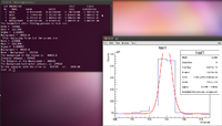
Now to find the error we can notice that the standard deviation here is 0.6238. The procedure is to expand the window by one or two standard deviations and find the difference in the number of counts in the original window. Due to the binning here I have decided to expand the window by 1 channel on each side, which is roughly 2 standard deviations. A picture is given below.
Now we do a similar method to find the number of counts within this window.
Now take the difference between the original window's number of counts and the expanded window's number of counts.
Now to propagate this error we must divide this number by the original number of counts.
This method was repeated for the next set of runs that make the data file. The numbers are in a table below.
| 0 <t< 300 sec | 730 < t < 1020 sec | 1480 < t < 1775 | 2250 < t < 2550 sec | 3050 < t < 3300 sec | 3775 < t < 4050 sec | 4480 < t < 4770 sec | ||
| Original Window Counts | 880200 | 716200 | 617100 | 545800 | 394100 | 362000 | 346300 | |
| Original Window Background (Integrated) | 381379 | 267608 | 215260 | 189665 | 143921 | 137541 | 128197 | |
| Original Window Difference | 498821 | 448592 | 401850 | 356135 | 250179 | 224459 | 218103 | |
| Expanded Window Counts | 970900 | 782600 | 671300 | 593100 | 426700 | 395400 | 378100 | |
| Expanded Window Background | 468138 | 333633 | 269025 | 236476 | 173353 | 170089 | 159644 | |
| Expanded Window Difference | 502762 | 448967 | 402275 | 356624 | 253347 | 225311 | 218456 | |
| Error in counts | 3941 | 375 | 425 | 489 | 3168 | 852 | 353 | |
| .dat file entry | 7.416220118 +/- 0.0079006297 | 7.343988145 +/- 0.0008359489264 | 7.216858801 +/- 0.0010576086 | 7.079282677 +/- 0.0013730748 | 6.908471023 +/- 0.012662933 | 6.704677244 +/- 0.0037957934 | 6.622841784 +/- 0.0016185014 |
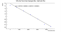
Below is the graph that contains the information about the initial activity and the half life
The slope of the line is -0.00019198 +/- 4.13511e^-7, which gives a half life of
While the error is
The constant value given by the plot is 7.4918 +/- 0.000927611, which gives an initial activity of
and an error of
Now correcting for the efficiency we have
While the error is
Below are the related pages for this sample using this method of window expansion:
Se170063 Nickel Foil Wide Gauss Window Expansion
Se170063 Pure Se Wide Gauss Window Expansion
Runlist
Table with dates and filename and locations on daq1


