Difference between revisions of "DV RunGroupC Moller"
(→Step 1) |
|||
| (605 intermediate revisions by 2 users not shown) | |||
| Line 1: | Line 1: | ||
| − | + | need to insert moller shielding into card after moller LUND file is created. (see clas12/beamline) | |
| − | = | + | Simulating the Moller scattering background for EG12 |
| + | =Docker= | ||
| + | ==[[Set up Docker Container]]== | ||
| + | =[[DV_XSECT|Moller Differential Cross-Section]]= | ||
| − | + | =GEANT4 Simulation of Moller Events= | |
| − | + | == [[LH2 target|Simulation Setup]]== | |
| + | Use GEANT4 via GEMC to estimate the Moller background for electron scattering experiments in JLab's Hall B. The first step towards this goal is to use GEANT4 without the GEMC infrastructure to create event (LUND) files that will be used as input events for GEMC. | ||
| − | + | ==[[DV_Moller_LH2 | Benchmark GEANT4's Moller scattering prediction with the theoretical cross section using LH2]]== | |
| − | |||
| − | |||
| − | |||
| − | |||
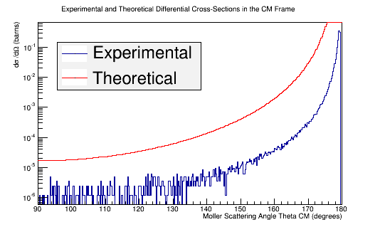
| − | + | ===Comparison of simulation vs. the theoretical Møller differential cross section using 11 GeV electrons impinging LH2=== | |
| − | + | [[Converting to barns|Converting the number of scattered electrons per scattering angle theta to a differential cross-section in barns.]] | |
| − | '' | + | [[File:XSect_new_zoom.png|frame|center|alt=Experimental and Theoretical Moller Differential Cross-Section in Center of Mass Frame Frame|'''Figure 5c:''' The experimental and theoretical Moller electron differential cross-section for an incident 11 GeV(Lab) electron in the Center of Mass frame of reference.]] |
| − | + | =Change to a NH3 Target= | |
| + | [[Replacing the LH2 target with an NH3 target]] | ||
| − | + | ==[[DV_Moller_NH3|Benchmark GEANT4's Moller scattering prediction with the theoretical cross section using NH3]]== | |
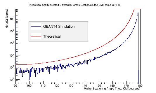
| − | + | ==Comparison of simulation vs. the theoretical Møller differential cross section using 11 GeV electrons impinging NH3== | |
| − | + | [[Converting to barns|Converting the number of scattered electrons per scattering angle theta to a differential cross-section in barns.]] | |
| − | '' | + | [[File:XSect_NH3.png|frame|center|alt=Theoretical and Simulated Moller Differential Cross-Section in Center of Mass Frame Frame|'''Figure 5c:''' The theoretical and simulated Moller electron differential cross-section for an incident 11 GeV(Lab) electron in the Center of Mass frame of reference for NH3 target.]] |
| − | + | ==LH2 Vs. NH3== | |
| + | ===[[DV_Moller_NH3_LH2|Benchmark GEANT4's Moller scattering prediction for NH3 and LH2]]=== | ||
| − | |||
| − | + | ==Effects Due to Target Material== | |
| + | ===[[DV_Target_Density|Target Density]]=== | ||
| − | |||
| − | + | ===[[DV_a_z_target|Atomic Mass and Electron Number Effects]]=== | |
| + | ==[[Calculating the differential cross-sections for the different materials, and placing them as well as the theoretical differential cross-section into a plot:|Differential Cross-Section Offset]]== | ||
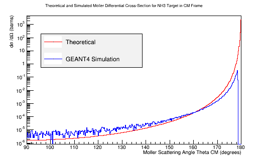
| − | [[File: | + | [[File:Adjusted_MollerXSect_NH3.png|frame|center|alt=Theoretical and Simulated Moller Differential Cross-Section in Center of Mass Frame Frame|'''Figure 5c:''' The theoretical and simulated Moller electron differential cross-section for an incident 11 GeV(Lab) electron in the Center of Mass frame of reference for NH3 target. The theoretical differential cross-section has been adjusted to account for the 10 electrons within NH3.]] |
| − | [[ | + | [[ROOT Macro to read LUND files and make plots]] |
| − | |||
| − | + | <center>[[File:LUND_MolMomCM.png]][[File:LUND_MolThetaCM.png]]</center> | |
| − | |||
| − | < | + | <center>[[File:LUND_MolMomLab.png]][[File:LUND_MolThetaLab.png]]</center> |
| − | |||
| − | |||
| − | |||
| − | + | Run the above theta and E distribution of Mollers through GEMC with and without Solenoid on. Determine the Theta and E range of Mollers that enter the detector. | |
| − | |||
| + | Scanning from 2MeV to 5500MeV, and 0 to 36 degrees in Theta. | ||
| − | + | For Solenoid on with 5T: | |
| − | + | <pre> | |
| + | <gcard> | ||
| + | |||
| + | <detector name="../../../../../clas12/fc/forwardCarriage" factory="TEXT" variation="original"/> | ||
| + | <detector name="../../../../../clas12/dc/dc" factory="TEXT" variation="original"/> | ||
| + | <detector name="../../../../../clas12/ec/ec" factory="TEXT" variation="original"/> | ||
| + | <detector name="../../../../../clas12/ctof/ctof" factory="TEXT" variation="original"/> | ||
| + | <detector name="../../../../../clas12/ftof/ftof" factory="TEXT" variation="original"/> | ||
| + | <detector name="../../../../../clas12/htcc/htcc" factory="TEXT" variation="original"/> | ||
| + | <detector name="../../../../../clas12/pcal/pcal" factory="TEXT" variation="original"/> | ||
| + | <option name="BEAM_P" value="e-, 2.800*GeV, 18.0*deg, 10*deg"/> | ||
| + | <option name="SPREAD_P" value="2.798*GeV, 18*deg, 180*deg"/> | ||
| + | <option name="SCALE_FIELD" value="clas12-torus-big, -1.0"/> | ||
| + | <option name="HALL_FIELD" value="clas12-solenoid"/> | ||
| + | <option name="SCALE_FIELD" value="clas12-solenoid, 1.0"/> | ||
| + | <option name="OUTPUT" value="evio,eg12.ev"/> | ||
| + | |||
| + | </gcard> | ||
| + | |||
| + | </pre> | ||
| + | |||
| + | Using the standard commands for gemc | ||
| + | |||
| + | <pre> | ||
| + | gemc -USE_GUI=0 -N=1000 eg12_sol.gcard | ||
| + | ~/src/CLAS/coatjava-1.0/bin/clas12-reconstruction -i eg12.ev -config DCHB::torus=-1.0 -config DCHB::solenoid=1.0 -config DCTB::kalman=true -o eg12_rec.ev -s DCHB:DCTB:EC:FTOF:EB | ||
| + | ~/src/CLAS/coatjava-1.0/bin/run-groovy Analysis.groovy eg12_rec.0.evio | ||
| + | </pre> | ||
| + | |||
| + | |||
| + | Checking for a reconstructed particle that undergoes a phi shift where the 1st column is energy and the 2nd the scattering angle theta: | ||
| + | <pre> | ||
| + | For Energy: | ||
| + | awk 'NR == 1 {line =$0; min =$2} NR >1 && $2 < min {line =$0; min = $2} END{print line}' Energy_Phi_Shift.dat | ||
| + | 289 0.6624017631112946 33.37507824033966 -179.63657653407975 0.7254709 29.696417 -177.79057 473.36051689004984 11.978802748439216 -129.55774724876173 | ||
| + | |||
| + | |||
| + | awk 'NR == 1 {line =$0; max =$2} NR >1 && $2 > max {line =$0; max = $2} END{print line}' Energy_Phi_Shift.dat | ||
| + | 978 5.584765946130235 24.90893565820338 -170.69784116534063 5.593401 24.90894 -170.65994 472.16552666546283 23.31807917059094 -165.11125601370114 | ||
| + | |||
| + | For Theta: | ||
| + | awk 'NR == 1 {line =$0; min =$3} NR >1 && $3 < min {line =$0; min = $3} END{print line}' Energy_Phi_Shift.dat | ||
| + | 12 4.83485521395583 10.577021312967325 -50.86708775351051 4.8205996 10.617784 -50.895683 491.627055439108 5.9032309421001985 -43.82964507576243 | ||
| + | |||
| + | awk 'NR == 1 {line =$0; max =$3} NR >1 && $3 > max {line =$0; max = $3} END{print line}' Energy_Phi_Shift.dat | ||
| + | 187 1.3382869250001856 35.63598792463312 29.887530073265214 1.3481133 35.449417 30.009071 472.455052447561 19.034043420497742 55.20328358414997 | ||
| + | </pre> | ||
| + | |||
| + | |||
| + | Similarly for 0T: | ||
| + | <pre> | ||
| + | For Energy: | ||
| + | awk 'NR == 1 {line =$0; min =$2} NR >1 && $2 < min {line =$0; min = $2} END{print line}' Energy_Phi_Shift.dat | ||
| + | 148 0.36418038435234207 33.68296595663359 -175.89942431595827 0.35383263 51.743824 -39.45801 469.5694572319308 24.353383233947522 -176.27025218702502 | ||
| + | |||
| + | |||
| + | awk 'NR == 1 {line =$0; max =$2} NR >1 && $2 > max {line =$0; max = $2} END{print line}' Energy_Phi_Shift.dat | ||
| + | 818 5.5278794590742235 12.937136966282836 -43.35663621477178 5.539351 12.95216 -49.09295 484.8800252169308 8.27731670021694 -43.245753766203364 | ||
| + | |||
| + | For Theta: | ||
| + | awk 'NR == 1 {line =$0; min =$3} NR >1 && $3 < min {line =$0; min = $3} END{print line}' Energy_Phi_Shift.dat | ||
| + | 559 4.909449160222199 9.918634647646794 0.06548256930681198 4.914272 9.938521 -5.861595 492.1448533455858 7.501204563534799 -0.006721611135017764 | ||
| + | |||
| + | awk 'NR == 1 {line =$0; max =$3} NR >1 && $3 > max {line =$0; max = $3} END{print line}' Energy_Phi_Shift.dat | ||
| + | 326 1.272966353429713 35.731680814303196 85.3173707349696 1.2830343 38.27654 58.368687 483.4835073848272 3.950855595379657 83.87603767806992 | ||
| + | </pre> | ||
| + | |||
| + | =Reconstruction of Moller Events= | ||
| + | |||
| + | ==[[DV_Creating_LUND_Files|The LUND format]]== | ||
| + | |||
| + | ==[[DV_Running_LUND_for_Moller_Distribution|Writing LUND files]]== | ||
| + | |||
| + | ==[[DV_Running_GEMC|Running GEMC]]== | ||
| + | |||
| + | ==[[DV_Analyze_Recon|Phi Shift observation using DC hit Reconstruction Data]]== | ||
| + | |||
| + | =Gcard creation defining energy and angle range of electrons= | ||
| + | ==[[Modified gcards]]== | ||
| + | |||
| + | =Effects of Solenoid on Electrons= | ||
| + | ==[[Results for known Moller events|Results for defined distribution in Solenoid Fields]]== | ||
| + | |||
| + | ==[[Results for Random Spread of Energy and angle theta in the Lab frame]]== | ||
| + | |||
| + | =Cover Full Solid Angle of Detector= | ||
| + | |||
| + | ==Using GEANT simulation data== | ||
| + | ===[[Calculations of 4-momentum components]]=== | ||
| + | |||
| + | ===[[Alter Phi Angles]]=== | ||
| + | |||
| + | ===[[Check Differential Cross-Section]]=== | ||
| + | |||
| + | |||
| + | |||
| + | |||
| + | ==Detector Occupancy== | ||
| + | |||
| + | clas12->Draw("Detector.wire:Detector.layer>>(7,1,7,120,0,120)","Detector.superlayer<3","colz") | ||
| + | |||
| + | ===[[gcard settings for daughter and procID|Gcard settings]]=== | ||
| + | |||
| + | ===[[Verfication of Mother/Daughter Occupancy]]=== | ||
| + | |||
| + | ===[[Benchmark GEMC Occupancy Prediction for 11GeV Electron Beam with 0T Solenoid for LH2]]=== | ||
| + | |||
| + | |||
| + | ===[[Setup for Batch Job With Varying Experimental CLAS12 Quantities]]=== | ||
| + | ===[[Run_in_GEMC]]=== | ||
| + | ===[[Center_of_Mass_for_Stationary_Target]]=== | ||
| + | |||
| + | ===[[Run Occupancy for Sector 1 DC hits]]=== | ||
| + | |||
| + | ===[[Wire_angle_correspondance]]=== | ||
| + | ===[[Isotropic Weighted Moller Distribution in GEMC]]=== | ||
=Papers used= | =Papers used= | ||
| − | |||
| − | An investigation of the spin structure of the proton in deep inelastic scattering of polarized muons on polarized protons [[:File:1819.pdf]] | + | [1]Farrukh Azfar's Derivation of Moller Scattering |
| + | |||
| + | :::[[File:FarrukAzfarMollerScatter.pdf]] | ||
| + | |||
| + | A polarized target for the CLAS detector | ||
| + | |||
| + | :::[[File:PHY02-33.pdf]] | ||
| + | |||
| + | An investigation of the spin structure of the proton in deep inelastic scattering of polarized muons on polarized protons | ||
| + | |||
| + | :::[[:File:1819.pdf]] | ||
| + | |||
| + | ==QED Radiative Corrections to Low-Energy Moller and Bhabha Scattering== | ||
| + | http://arxiv.org/abs/1602.07609 | ||
| + | |||
| + | [[File:ChangingRates_S1_PhiThetaHits.png | 600 px]] | ||
| + | |||
| + | [[File:S1_50nA_PrimaryElectronSigmasWeightedRates.png | 600 px]] | ||
| + | |||
| + | [[File:S1_PhiThetaGammaHits.png | 600 px]] | ||
| + | |||
| + | |||
| + | [[File:HitMakeUp.png]] | ||
| + | |||
| + | |||
| + | [[File:S1_50nA_PrimaryElectronSigmasWeightedRates_Full.png | 600 px]] | ||
| + | |||
| + | [[File:ComparingOppositeFields_S1_PhiThetaHits.png | 800 px]] | ||
| + | |||
| + | |||
| + | [[File:ChangingSolenoidRates_wo_Magnets.png|800 px]] | ||
| + | |||
| + | |||
| + | [[File:ComparingDCcomponents_S1_PhiThetaHits.png| 800 px]] | ||
| + | |||
| + | |||
| + | |||
| + | [[File:ComparingDCEndplates_S1_PhiThetaHits.png | 800 px]] | ||
| + | |||
| + | |||
| + | [[File:ComparingMagnetComponents_S1_PhiThetaHits.png| 800 px]] | ||
| + | |||
| + | [[File:S1_PhiThetaGammaHits_Full.png | 600 px]] | ||
| + | |||
| + | |||
| + | |||
| + | |||
| + | Tomography | ||
| + | |||
| + | [[File:S1_PhiThetaGammaVertex_wo_MagnetComponents.png | 600 px]] | ||
| + | |||
| + | |||
| + | =GEANT4 Simulation of Lead Conic Moller Shield= | ||
| + | ==[[Lead Shield Cone]]== | ||
| + | |||
| + | ====OLD==== | ||
| + | {| class="wikitable" | ||
| + | |+ FTOn from Forward Vertex | ||
| + | ! 50nA | ||
| + | ! S1R1 2ndryMoller e- rate | ||
| + | ! S1R1 2ndryMoller gamma rate | ||
| + | ! S1R1 2ndryMoller particle rate | ||
| + | ! Effective Shield Rate | ||
| + | |- | ||
| + | ! R1_36_38_R2_36_38 | ||
| + | | ? | ||
| + | | ? | ||
| + | | ? | ||
| + | | ? | ||
| + | |||
| + | |} | ||
| + | {| class="wikitable" | ||
| + | |+ OLD! FTOn from 0,0,0 Vertex | ||
| + | ! 50nA | ||
| + | ! S1R1 2ndryMoller e- rate | ||
| + | ! S1R1 2ndryMoller gamma rate | ||
| + | ! S1R1 2ndryMoller particle rate | ||
| + | ! Effective Shield Rate | ||
| + | |- | ||
| + | ! R1_36_38_R2_36_38 | ||
| + | | 405 Hz | ||
| + | | 15480 Hz | ||
| + | | 160 Hz | ||
| + | | ? | ||
| + | |- | ||
| + | ! R1_36_38_R2_50_52 | ||
| + | | 470 Hz | ||
| + | | 15227 Hz | ||
| + | | 146 Hz | ||
| + | | ? | ||
| + | |- | ||
| + | ! R1_36_38_R2_70_72 | ||
| + | | 461 Hz | ||
| + | | 15045 Hz | ||
| + | | 150 Hz | ||
| + | | ? | ||
| + | |- | ||
| + | ! R1_36_38_R2_75_77 | ||
| + | | 372 Hz | ||
| + | | 14916 Hz | ||
| + | | 130 Hz | ||
| + | | ? | ||
| + | |- | ||
| + | ! R1_36_38_R2_80_82 | ||
| + | | 376 Hz | ||
| + | | 14995 Hz | ||
| + | | 109 Hz | ||
| + | | ? | ||
| + | |- | ||
| + | ! R1_36_38_R2_90_92 | ||
| + | | 413 Hz | ||
| + | | 14580 Hz | ||
| + | | 119 Hz | ||
| + | | ? | ||
| + | |- | ||
| + | ! R1_36_38_R2_95_97 | ||
| + | | 383 Hz | ||
| + | | 14186 Hz | ||
| + | | 117 Hz | ||
| + | | ? | ||
| + | |- | ||
| + | ! R1_36_38_R2_111_113 | ||
| + | | 447 Hz | ||
| + | | 14196 Hz | ||
| + | | 109 Hz | ||
| + | | ? | ||
| + | |- | ||
| + | ! R1_36_38_R2_116_118 | ||
| + | | 420 Hz | ||
| + | | 14167 Hz | ||
| + | | 144 Hz | ||
| + | | ? | ||
| + | |- | ||
| + | ! R1_36_38_R2_121_123 | ||
| + | | 389 Hz | ||
| + | | 14251 Hz | ||
| + | | 117 Hz | ||
| + | | ? | ||
| + | |- | ||
| + | ! R1_74_76_R2_151_153 | ||
| + | | 492 Hz | ||
| + | | 14280 Hz | ||
| + | | 110 Hz | ||
| + | | ? | ||
| + | |- | ||
| + | ! R1_36_38_R2_500_503 | ||
| + | | 1000 Hz | ||
| + | | 18363 Hz | ||
| + | | 120 Hz | ||
| + | | ? | ||
| + | |} | ||
| + | |||
| + | {| class="wikitable" | ||
| + | |+ FTOn from (0,0,0) Vertex w/o FT | ||
| + | ! 50nA | ||
| + | ! S1R1 2ndryMoller e- rate | ||
| + | ! S1R1 2ndryMoller gamma rate | ||
| + | ! S1R1 2ndryMoller particle rate | ||
| + | ! Effective Shield Rate | ||
| + | |- | ||
| + | ! R1_0_524.0_R2_0_1034.47 | ||
| + | | ? | ||
| + | | ? | ||
| + | | ? | ||
| + | | ? | ||
| + | |||
| + | |} | ||
| + | |||
| + | {| class="wikitable" | ||
| + | |+ FTOn from Forward Vertex | ||
| + | ! 50nA | ||
| + | ! S1R1 2ndryMoller e- rate | ||
| + | ! S1R1 2ndryMoller gamma rate | ||
| + | ! S1R1 2ndryMoller particle rate | ||
| + | ! Effective Shield Rate | ||
| + | |- | ||
| + | ! R1_36_38_R2_36_38 | ||
| + | | ? | ||
| + | | ? | ||
| + | | ? | ||
| + | | ? | ||
| + | |||
| + | |} | ||
| + | |||
| + | |||
| + | [[VanWasshenova_Thesis]] | ||
[[EG12]] | [[EG12]] | ||
Latest revision as of 18:03, 13 January 2019
need to insert moller shielding into card after moller LUND file is created. (see clas12/beamline)
Simulating the Moller scattering background for EG12
Docker
Set up Docker Container
Moller Differential Cross-Section
GEANT4 Simulation of Moller Events
Simulation Setup
Use GEANT4 via GEMC to estimate the Moller background for electron scattering experiments in JLab's Hall B. The first step towards this goal is to use GEANT4 without the GEMC infrastructure to create event (LUND) files that will be used as input events for GEMC.
Benchmark GEANT4's Moller scattering prediction with the theoretical cross section using LH2
Comparison of simulation vs. the theoretical Møller differential cross section using 11 GeV electrons impinging LH2
Change to a NH3 Target
Replacing the LH2 target with an NH3 target
Benchmark GEANT4's Moller scattering prediction with the theoretical cross section using NH3
Comparison of simulation vs. the theoretical Møller differential cross section using 11 GeV electrons impinging NH3
LH2 Vs. NH3
Benchmark GEANT4's Moller scattering prediction for NH3 and LH2
Effects Due to Target Material
Target Density
Atomic Mass and Electron Number Effects
Differential Cross-Section Offset
ROOT Macro to read LUND files and make plots
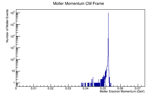
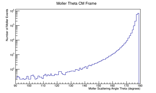
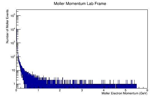
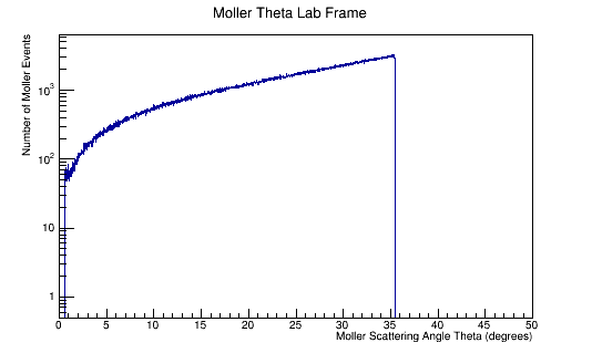
Run the above theta and E distribution of Mollers through GEMC with and without Solenoid on. Determine the Theta and E range of Mollers that enter the detector.
Scanning from 2MeV to 5500MeV, and 0 to 36 degrees in Theta.
For Solenoid on with 5T:
<gcard>

        <detector name="../../../../../clas12/fc/forwardCarriage" factory="TEXT" variation="original"/>
        <detector name="../../../../../clas12/dc/dc"            factory="TEXT" variation="original"/>
        <detector name="../../../../../clas12/ec/ec"            factory="TEXT" variation="original"/>
        <detector name="../../../../../clas12/ctof/ctof"            factory="TEXT" variation="original"/>
        <detector name="../../../../../clas12/ftof/ftof"            factory="TEXT" variation="original"/>
        <detector name="../../../../../clas12/htcc/htcc"            factory="TEXT" variation="original"/>
        <detector name="../../../../../clas12/pcal/pcal"            factory="TEXT" variation="original"/>
        <option name="BEAM_P"   value="e-, 2.800*GeV, 18.0*deg, 10*deg"/>
        <option name="SPREAD_P" value="2.798*GeV, 18*deg, 180*deg"/>
        <option name="SCALE_FIELD" value="clas12-torus-big, -1.0"/>
        <option name="HALL_FIELD"  value="clas12-solenoid"/>
        <option name="SCALE_FIELD" value="clas12-solenoid, 1.0"/>
        <option name="OUTPUT" value="evio,eg12.ev"/>

</gcard>
Using the standard commands for gemc
gemc -USE_GUI=0 -N=1000 eg12_sol.gcard
~/src/CLAS/coatjava-1.0/bin/clas12-reconstruction -i eg12.ev -config DCHB::torus=-1.0 -config DCHB::solenoid=1.0 -config DCTB::kalman=true -o eg12_rec.ev -s DCHB:DCTB:EC:FTOF:EB
~/src/CLAS/coatjava-1.0/bin/run-groovy Analysis.groovy eg12_rec.0.evio
Checking for a reconstructed particle that undergoes a phi shift where the 1st column is energy and the 2nd the scattering angle theta:
For Energy:
awk 'NR == 1 {line =$0; min =$2} NR >1 && $2 < min {line =$0; min = $2} END{print line}' Energy_Phi_Shift.dat
289     0.6624017631112946      33.37507824033966       -179.63657653407975     0.7254709       29.696417       -177.79057      473.36051689004984      11.978802748439216      -129.55774724876173


awk 'NR == 1 {line =$0; max =$2} NR >1 && $2 > max {line =$0; max = $2} END{print line}' Energy_Phi_Shift.dat
978     5.584765946130235       24.90893565820338       -170.69784116534063     5.593401        24.90894        -170.65994      472.16552666546283      23.31807917059094       -165.11125601370114

For Theta:
awk 'NR == 1 {line =$0; min =$3} NR >1 && $3 < min {line =$0; min = $3} END{print line}' Energy_Phi_Shift.dat
12      4.83485521395583        10.577021312967325      -50.86708775351051      4.8205996       10.617784       -50.895683      491.627055439108        5.9032309421001985      -43.82964507576243

awk 'NR == 1 {line =$0; max =$3} NR >1 && $3 > max {line =$0; max = $3} END{print line}' Energy_Phi_Shift.dat
187     1.3382869250001856      35.63598792463312       29.887530073265214      1.3481133       35.449417       30.009071       472.455052447561        19.034043420497742      55.20328358414997
Similarly for 0T:
For Energy:
awk 'NR == 1 {line =$0; min =$2} NR >1 && $2 < min {line =$0; min = $2} END{print line}' Energy_Phi_Shift.dat
148     0.36418038435234207     33.68296595663359       -175.89942431595827     0.35383263      51.743824       -39.45801       469.5694572319308       24.353383233947522      -176.27025218702502


awk 'NR == 1 {line =$0; max =$2} NR >1 && $2 > max {line =$0; max = $2} END{print line}' Energy_Phi_Shift.dat
818     5.5278794590742235      12.937136966282836      -43.35663621477178      5.539351        12.95216        -49.09295       484.8800252169308       8.27731670021694        -43.245753766203364

For Theta:
awk 'NR == 1 {line =$0; min =$3} NR >1 && $3 < min {line =$0; min = $3} END{print line}' Energy_Phi_Shift.dat
559     4.909449160222199       9.918634647646794       0.06548256930681198     4.914272        9.938521        -5.861595       492.1448533455858       7.501204563534799       -0.006721611135017764

awk 'NR == 1 {line =$0; max =$3} NR >1 && $3 > max {line =$0; max = $3} END{print line}' Energy_Phi_Shift.dat
326     1.272966353429713       35.731680814303196      85.3173707349696        1.2830343       38.27654        58.368687       483.4835073848272       3.950855595379657       83.87603767806992
Reconstruction of Moller Events
The LUND format
Writing LUND files
Running GEMC
Phi Shift observation using DC hit Reconstruction Data
Gcard creation defining energy and angle range of electrons
Modified gcards
Effects of Solenoid on Electrons
Results for defined distribution in Solenoid Fields
Results for Random Spread of Energy and angle theta in the Lab frame
Cover Full Solid Angle of Detector
Using GEANT simulation data
Calculations of 4-momentum components
Alter Phi Angles
Check Differential Cross-Section
Detector Occupancy
clas12->Draw("Detector.wire:Detector.layer>>(7,1,7,120,0,120)","Detector.superlayer<3","colz")
Gcard settings
Verfication of Mother/Daughter Occupancy
Benchmark GEMC Occupancy Prediction for 11GeV Electron Beam with 0T Solenoid for LH2
Setup for Batch Job With Varying Experimental CLAS12 Quantities
Run_in_GEMC
Center_of_Mass_for_Stationary_Target
Run Occupancy for Sector 1 DC hits
Wire_angle_correspondance
Isotropic Weighted Moller Distribution in GEMC
Papers used
[1]Farrukh Azfar's Derivation of Moller Scattering
A polarized target for the CLAS detector
An investigation of the spin structure of the proton in deep inelastic scattering of polarized muons on polarized protons
QED Radiative Corrections to Low-Energy Moller and Bhabha Scattering
http://arxiv.org/abs/1602.07609
Tomography
GEANT4 Simulation of Lead Conic Moller Shield
Lead Shield Cone
OLD
| 50nA | S1R1 2ndryMoller e- rate | S1R1 2ndryMoller gamma rate | S1R1 2ndryMoller particle rate | Effective Shield Rate |
|---|---|---|---|---|
| R1_36_38_R2_36_38 | ? | ? | ? | ? |
| 50nA | S1R1 2ndryMoller e- rate | S1R1 2ndryMoller gamma rate | S1R1 2ndryMoller particle rate | Effective Shield Rate |
|---|---|---|---|---|
| R1_36_38_R2_36_38 | 405 Hz | 15480 Hz | 160 Hz | ? |
| R1_36_38_R2_50_52 | 470 Hz | 15227 Hz | 146 Hz | ? |
| R1_36_38_R2_70_72 | 461 Hz | 15045 Hz | 150 Hz | ? |
| R1_36_38_R2_75_77 | 372 Hz | 14916 Hz | 130 Hz | ? |
| R1_36_38_R2_80_82 | 376 Hz | 14995 Hz | 109 Hz | ? |
| R1_36_38_R2_90_92 | 413 Hz | 14580 Hz | 119 Hz | ? |
| R1_36_38_R2_95_97 | 383 Hz | 14186 Hz | 117 Hz | ? |
| R1_36_38_R2_111_113 | 447 Hz | 14196 Hz | 109 Hz | ? |
| R1_36_38_R2_116_118 | 420 Hz | 14167 Hz | 144 Hz | ? |
| R1_36_38_R2_121_123 | 389 Hz | 14251 Hz | 117 Hz | ? |
| R1_74_76_R2_151_153 | 492 Hz | 14280 Hz | 110 Hz | ? |
| R1_36_38_R2_500_503 | 1000 Hz | 18363 Hz | 120 Hz | ? |
| 50nA | S1R1 2ndryMoller e- rate | S1R1 2ndryMoller gamma rate | S1R1 2ndryMoller particle rate | Effective Shield Rate |
|---|---|---|---|---|
| R1_0_524.0_R2_0_1034.47 | ? | ? | ? | ? |
| 50nA | S1R1 2ndryMoller e- rate | S1R1 2ndryMoller gamma rate | S1R1 2ndryMoller particle rate | Effective Shield Rate |
|---|---|---|---|---|
| R1_36_38_R2_36_38 | ? | ? | ? | ? |
