|
|
| Line 3: |
Line 3: |
| | =[[TD_Ddoverd_2010]]= | | =[[TD_Ddoverd_2010]]= |
| | =[[TD_Ddoverd_2011]]= | | =[[TD_Ddoverd_2011]]= |
| − |
| |
| − |
| |
| − | =5-01-2009=
| |
| − |
| |
| − | ==Target and Beam Polarization are positive==
| |
| − |
| |
| − |
| |
| − | {| border="1" |cellpadding="20" cellspacing="0
| |
| − | |-
| |
| − | | Helcode # || Negative Beam Torus || Positive Beam Torus
| |
| − | |-
| |
| − | | 1 h>0|| [[Image:BT_negative_&_helcode_1_phi_angle_cm_frame_PbPt_positive.gif|300px]] || [[Image:BT_positive_&_helcode_1_phi_angle_cm_frame_PbPt_positive.gif|300px]]
| |
| − | |-
| |
| − | | 2 h<0|| [[Image:BT_negative_&_helcode_2_phi_angle_cm_frame_PbPt_positive.gif|300px]] || [[Image:BT_positive_&_helcode_2_phi_angle_cm_frame_PbPt_positive.gif|300px]]
| |
| − | |-
| |
| − | | 3 || [[Image:BT_negative_&_helcode_3_phi_angle_cm_frame_PbPt_positive.gif|300px]] || [[Image:BT_positive_&_helcode_3_phi_angle_cm_frame_PbPt_positive.gif|300px]]
| |
| − | |-
| |
| − | | 4 || [[Image:BT_negative_&_helcode_4_phi_angle_cm_frame_PbPt_positive.gif|300px]] || [[Image:BT_positive_&_helcode_4_phi_angle_cm_frame_PbPt_positive.gif|300px]]
| |
| − | |}<br>
| |
| − |
| |
| − |
| |
| − | ===Target Polarization Positive and Beam Polarization Negative===
| |
| − |
| |
| − |
| |
| − | {| border="1" |cellpadding="20" cellspacing="0
| |
| − | |-
| |
| − | | Helcode # || Negative Beam Torus || Positive Beam Torus
| |
| − | |-
| |
| − | | 1 h>0|| No Data || [[Image:BT_positive_&_helcode_1_phi_angle_cm_frame_Pt_positive_Pb_negative.gif|300px]]
| |
| − | |-
| |
| − | | 2 h<0|| No Data || [[Image:BT_positive_&_helcode_2_phi_angle_cm_frame_Pt_positive_Pb_negative.gif|300px]]
| |
| − | |-
| |
| − | | 3 || No Data|| [[Image:BT_positive_&_helcode_3_phi_angle_cm_frame_Pt_positive_Pb_negative.gif|300px]]
| |
| − | |-
| |
| − | | 4 || No Data || [[Image:BT_positive_&_helcode_4_phi_angle_cm_frame_Pt_positive_Pb_negative.gif|300px]]
| |
| − | |}<br>
| |
| − |
| |
| − | ===Inclusive Histograms For Invariant Mass===
| |
| − | ====Invariant Mass Histograms for Each Sector====
| |
| − |
| |
| − | =====All helicities=====
| |
| − |
| |
| − | [[Image:InvariantMass_sector_1.gif|300px]][[Image:InvariantMass_sector_2.gif|300px]]<br>
| |
| − | [[Image:InvariantMass_sector_3.gif|300px]][[Image:InvariantMass_sector_4.gif|300px]]<br>
| |
| − | [[Image:InvariantMass_sector_5.gif|300px]][[Image:InvariantMass_sector_6.gif|300px]]<br>
| |
| − |
| |
| − |
| |
| − | [[Image:InvariantMass_sector_1_gaussian.gif|300px]][[Image:InvariantMass_sector_2_gaussian.gif|300px]]<br>
| |
| − | [[Image:InvariantMass_sector_3_gaussian.gif|300px]][[Image:InvariantMass_sector_4_gaussian.gif|300px]]<br>
| |
| − | [[Image:InvariantMass_sector_5_gaussian.gif|300px]][[Image:InvariantMass_sector_6_gaussian.gif|300px]]<br>
| |
| − |
| |
| − | =====Helcode=1=====
| |
| − |
| |
| − | [[Image:InvariantMass_sector_1_H1.gif|300px]][[Image:InvariantMass_sector_2_H1.gif|300px]]<br>
| |
| − | [[Image:InvariantMass_sector_3_H1.gif|300px]][[Image:InvariantMass_sector_4_H1.gif|300px]]<br>
| |
| − | [[Image:InvariantMass_sector_5_H1.gif|300px]][[Image:InvariantMass_sector_6_H1.gif|300px]]<br>
| |
| − |
| |
| − | =3/20/09=
| |
| − |
| |
| − | [[Image:InvariantMass_W_difference_Coupleoffiles_26992.gif|450px]]
| |
| − |
| |
| − | [[Image:InvariantMass_W_difference_Coupleoffiles_26993.gif|450px]]
| |
| − |
| |
| − | [[Image:InvariantMass_W_difference_Coupleoffiles_26994.gif|450px]]
| |
| − |
| |
| − | 1.) plot Wdiff
| |
| − |
| |
| − | 2.) plot PE using Osipenko/Josh cuts
| |
| − |
| |
| − |
| |
| − |
| |
| − |
| |
| − |
| |
| − |
| |
| − |
| |
| − | =06/6/09=
| |
| − |
| |
| − | ==Invariant Mass==
| |
| − |
| |
| − | Difference of Invariant Mass for two differnet cuts:
| |
| − |
| |
| − | {| border="1" |cellpadding="20" cellspacing="0
| |
| − | |-
| |
| − | | Run Number || EC Cuts+ requiring pion || OSI Cuts || EC Cuts ||
| |
| − | |-
| |
| − | | 26991 || [[Image:Missing_mass_difference_RunNumber26991_1.gif|150px]] || [[Image:Missing_mass_difference_RunNumber26991_1_OSICuts.gif|150px]] ||
| |
| − | [[Image:Missing_mass_difference_RunNumber26991_1ECuts.gif|150px]]
| |
| − | |}
| |
| − |
| |
| − |
| |
| − | On x-axis of FC difference between the "+" heliciy FC and the "-" helicity FC.
| |
| − |
| |
| − | {| border="1" |cellpadding="20" cellspacing="0
| |
| − | |-
| |
| − | | Run Number || W difference || FC difference || End of Run sum <math>\equiv \frac {\sum_i(FC(i)^+) - \sum(FC(i)^-)}{\sum (FC(i)^+) + \sum(FC(i)^-)})</math>
| |
| − | |-
| |
| − | | 26991 || [[Image:Missing_mass_difference_RunNumber26991_1_OSICuts.gif|150px]] || [[Image:FC_difference_RunNumber26991_OSICuts.gif|150px]] ||0.00354260538 <math>\pm</math> 0.00001050400
| |
| − | |-
| |
| − | | 26994 || [[Image:Missing_mass_difference_RunNumber26994_1_OSICuts.gif|150px]] || [[Image:FC_difference_RunNumber26994_OSICuts.gif|150px]] || 0.00367 <math>\pm</math> 0.00001088263
| |
| − | |-
| |
| − | | 26993 || [[Image:Missing_mass_difference_RunNumber26993_1_OSICuts.gif|150px]] || [[Image:FC_difference_RunNumber26993_OSICuts.gif|150px]] || 0.002559223 <math>\pm</math> 0.00001120796
| |
| − | |-
| |
| − | | 26992 || [[Image:Missing_mass_difference_RunNumber26992_1_OSICuts.gif|150px]] || [[Image:FC_difference_RunNumber26992_OSICuts.gif|150px]] || 0.003781<math>\pm</math>0.00001090044
| |
| − | |-
| |
| − | | 26990 || [[Image:Missing_mass_difference_RunNumber26990_1_OSICuts.gif|150px]] || [[Image:FC_difference_RunNumber26990_OSICuts.gif|150px]] || 0.00331986321<math>\pm</math>0.00001203387
| |
| − | |-
| |
| − | | 26989 || [[Image:Missing_mass_difference_RunNumber26989_1_OSICuts.gif|150px]] || [[Image:FC_difference_RunNumber26989_OSICuts.gif|150px]] || 0.00303841557<math>\pm</math>0.00001267152
| |
| − | |-
| |
| − | | 26988 || [[Image:Missing_mass_difference_RunNumber26988_1_OSICuts.gif|150px]] || [[Image:FC_difference_RunNumber26988_OSICuts.gif|150px]] || 0.00380169243<math>\pm</math>0.00001097470
| |
| − | |-
| |
| − | | 26987 || [[Image:Missing_mass_difference_RunNumber26987_1_OSICuts.gif|150px]] || [[Image:FC_difference_RunNumber26987_OSICuts.gif|150px]] || 0.00280163240<math>\pm</math>0.00001515270
| |
| − | |-
| |
| − | | 26986 || [[Image:Missing_mass_difference_RunNumber26986_1_OSICuts.gif|150px]] || [[Image:FC_difference_RunNumber26986_OSICuts.gif|150px]] || 0.00352882616<math>\pm</math>0.00000048897
| |
| − | |-
| |
| − | | 26979 || [[Image:Missing_mass_difference_RunNumber26979_1_OSICuts.gif|150px]] || [[Image:FC_difference_RunNumber26979_OSICuts.gif|150px]] || -0.00373104126<math>\pm</math>0.00001531706
| |
| − | |-
| |
| − | | 26965 || [[Image:Missing_mass_difference_RunNumber26965_1_OSICuts.gif|150px]] || [[Image:FC_difference_RunNumber26965_OSICuts.gif|150px]] || 0.00454140439<math>\pm</math>0.00001534923
| |
| − | |-
| |
| − | | 26964 || [[Image:Missing_mass_difference_RunNumber26964_1_OSICuts.gif|150px]] || [[Image:FC_difference_RunNumber26964_OSICuts.gif|150px]] || 0.00509434283<math>\pm</math>0.00001557226
| |
| − | |-
| |
| − | | 26963 || [[Image:Missing_mass_difference_RunNumber26963_1_OSICuts.gif|150px]] || [[Image:FC_difference_RunNumber26963_OSICuts.gif|150px]] || 0.00405285155<math>\pm</math>0.00001575049
| |
| − | |-
| |
| − | | 26961 || [[Image:Missing_mass_difference_RunNumber26961_1_OSICuts.gif|150px]] || [[Image:FC_difference_RunNumber26961_OSICuts.gif|150px]] || 0.00507456102 <math>\pm</math>0.00001682744
| |
| − | |-
| |
| − | | 26959 || [[Image:Missing_mass_difference_RunNumber26959_1_OSICuts.gif|150px]] || [[Image:FC_difference_RunNumber26959_OSICuts.gif|150px]] ||0.00523761694<math>\pm</math>0.00001488890
| |
| − | |-
| |
| − | | 26958 || [[Image:Missing_mass_difference_RunNumber26958_1_OSICuts.gif|150px]] || [[Image:FC_difference_RunNumber26958_OSICuts.gif|150px]] || 0.00444205478<math>\pm</math> 0.00001577510
| |
| − | |-
| |
| − | | 26956 || [[Image:Missing_mass_difference_RunNumber26956_1_OSICuts.gif|150px]] || [[Image:FC_difference_RunNumber26956_OSICuts.gif|150px]] ||0.00504401620<math>\pm</math>0.00001565456
| |
| − | |-
| |
| − | | 26955 || [[Image:Missing_mass_difference_RunNumber26955_1_OSICuts.gif|150px]] || [[Image:FC_difference_RunNumber26955_OSICuts.gif|150px]] || 0.00559913829<math>\pm</math>0.00001425736
| |
| − | |-
| |
| − | | 26954 || [[Image:Missing_mass_difference_RunNumber26954_1_OSICuts.gif|150px]] || [[Image:FC_difference_RunNumber26954_OSICuts.gif|150px]] || 0.00494690728<math>\pm</math>0.00001443107
| |
| − | |-
| |
| − | | 26953 || [[Image:Missing_mass_difference_RunNumber26953_1_OSICuts.gif|150px]] || [[Image:FC_difference_RunNumber26953_OSICuts.gif|150px]] || 0.00562598448<math>\pm</math>0.00001525797
| |
| − | |-
| |
| − | | 26952 || [[Image:Missing_mass_difference_RunNumber26952_1_OSICuts.gif|150px]] || [[Image:FC_difference_RunNumber26952_OSICuts.gif|150px]] || 0.00485295834<math>\pm</math>0.00001293033
| |
| − | |-
| |
| − | | 26951 || [[Image:Missing_mass_difference_RunNumber26951_1_OSICuts.gif|150px]] || [[Image:FC_difference_RunNumber26951_OSICuts.gif|150px]] || 0.00545485906<math>\pm</math>0.00001558637
| |
| − | |-
| |
| − | | 26947 || [[Image:Missing_mass_difference_RunNumber26947_1_OSICuts.gif|150px]] || [[Image:FC_difference_RunNumber26947_OSICuts.gif|150px]] || 0.00465697160<math>\pm</math>0.00001144285
| |
| − | |-
| |
| − | | 26945 || [[Image:Missing_mass_difference_RunNumber26945_1_OSICuts.gif|150px]] || [[Image:FC_difference_RunNumber26945_OSICuts.gif|150px]] ||-0.00556456389<math>\pm</math> 0.00001389870
| |
| − | |-
| |
| − | | 26943 || [[Image:Missing_mass_difference_RunNumber26943_1_OSICuts.gif|150px]] || [[Image:FC_difference_RunNumber26943_OSICuts.gif|150px]] ||-0.00656109472<math>\pm</math>0.00001540342
| |
| − | |-
| |
| − | | 26942 || [[Image:Missing_mass_difference_RunNumber26942_1_OSICuts.gif|150px]] || [[Image:FC_difference_RunNumber26942_OSICuts.gif|150px]] ||-0.00669169106<math>\pm</math>0.00001526771
| |
| − | |-
| |
| − | | 26941 || [[Image:Missing_mass_difference_RunNumber26941_1_OSICuts.gif|150px]] || [[Image:FC_difference_RunNumber26941_OSICuts.gif|150px]] || -0.00676460417<math>\pm</math>0.00001100372
| |
| − | |-
| |
| − | | 26940 || [[Image:Missing_mass_difference_RunNumber26940_1_OSICuts.gif|150px]] || [[Image:FC_difference_RunNumber26940_OSICuts.gif|150px]] || -0.00643597022 <math>\pm</math>0.00001397207
| |
| − | |-
| |
| − | | 26939 || [[Image:Missing_mass_difference_RunNumber26939_1_OSICuts.gif|150px]] || [[Image:FC_difference_RunNumber26939_OSICuts.gif|150px]] || -0.00650047456<math>\pm</math>0.00001405001
| |
| − | |-
| |
| − | | 26938 || [[Image:Missing_mass_difference_RunNumber26938_1_OSICuts.gif|150px]] || [[Image:FC_difference_RunNumber26938_OSICuts.gif|150px]] || -0.00632630313<math>\pm</math>0.00001411839
| |
| − | |-
| |
| − | | 26937 || [[Image:Missing_mass_difference_RunNumber26937_1_OSICuts.gif|150px]] || [[Image:FC_difference_RunNumber26937_OSICuts.gif|150px]] || -0.00533169794<math>\pm</math>0.00001417768
| |
| − | |-
| |
| − | | 26934 || [[Image:Missing_mass_difference_RunNumber26934_1_OSICuts.gif|150px]] || [[Image:FC_difference_RunNumber26934_OSICuts.gif|150px]] || -0.00601497156<math>\pm</math>0.00001422560
| |
| − | |-
| |
| − | | 26933 || [[Image:Missing_mass_difference_RunNumber26933_1_OSICuts.gif|150px]] || [[Image:FC_difference_RunNumber26933_OSICuts.gif|150px]] || -0.00586540500<math>\pm</math>0.00001414938
| |
| − | |-
| |
| − | | 26932 || [[Image:Missing_mass_difference_RunNumber26932_1_OSICuts.gif|150px]] || [[Image:FC_difference_RunNumber26932_OSICuts.gif|150px]] || -0.00587687192<math>\pm</math>0.00001383218
| |
| − | |-
| |
| − | | 26931 || [[Image:Missing_mass_difference_RunNumber26931_1_OSICuts.gif|150px]] || [[Image:FC_difference_RunNumber26931_OSICuts.gif|150px]] || -0.00630232566<math>\pm</math>0.00001495053
| |
| − | |-
| |
| − | | 26930 || [[Image:Missing_mass_difference_RunNumber26930_1_OSICuts.gif|150px]] || [[Image:FC_difference_RunNumber26930_OSICuts.gif|150px]] || -0.00684205010<math>\pm</math>0.00001541629
| |
| − | |-
| |
| − | | 26929 || [[Image:Missing_mass_difference_RunNumber26929_1_OSICuts.gif|150px]] || [[Image:FC_difference_RunNumber26929_OSICuts.gif|150px]] || -0.00521666944<math>\pm</math>0.00001555256
| |
| − | |-
| |
| − | | 26928 || [[Image:Missing_mass_difference_RunNumber26928_1_OSICuts.gif|150px]] || [[Image:FC_difference_RunNumber26928_OSICuts.gif|150px]] || -0.00682185316<math>\pm</math>0.00001536552
| |
| − | |-
| |
| − | | 26927 || [[Image:Missing_mass_difference_RunNumber26927_1_OSICuts.gif|150px]] || [[Image:FC_difference_RunNumber26927_OSICuts.gif|150px]] || -0.00599647483<math>\pm</math>0.00001538040
| |
| − | |-
| |
| − | | 26926 || [[Image:Missing_mass_difference_RunNumber26926_1_OSICuts.gif|150px]] || [[Image:FC_difference_RunNumber26926_OSICuts.gif|150px]] || -0.00649932378<math>\pm</math>0.00001302331
| |
| − | |-
| |
| − | | 26925 || [[Image:Missing_mass_difference_RunNumber26925_1_OSICuts.gif|150px]] || [[Image:FC_difference_RunNumber26925_OSICuts.gif|150px]] || -0.00575464099<math>\pm</math>0.00001530219
| |
| − | |-
| |
| − | | 27079 || [[Image:Missing_mass_difference_RunNumber27079_1_OSICuts.gif|150px]] || [[Image:FC_difference_RunNumber27079_OSICuts.gif|150px]] || -0.01025869470<math>\pm</math>0.00002322298
| |
| − | |-
| |
| − | | 27078 || [[Image:Missing_mass_difference_RunNumber27078_1_OSICuts.gif|150px]] || [[Image:FC_difference_RunNumber27078_OSICuts.gif|150px]] || -0.01128036266<math>\pm</math>0.00002135573
| |
| − | |-
| |
| − | | 27075 || [[Image:Missing_mass_difference_RunNumber27075_1_OSICuts.gif|150px]] || [[Image:FC_difference_RunNumber27075_OSICuts.gif|150px]] || -0.01037443017<math>\pm</math>0.00002113646
| |
| − | |-
| |
| − | | 27109|| [[Image:Missing_mass_difference_RunNumber27109_1_OSICuts.gif|150px]] || [[Image:FC_difference_RunNumber27109_OSICuts.gif|150px]] || -0.00876887465<math>\pm</math>0.00002411331
| |
| − | |-
| |
| − | | 27107|| [[Image:Missing_mass_difference_RunNumber27107_1_OSICuts.gif|150px]] || [[Image:FC_difference_RunNumber27107_OSICuts.gif|150px]] || 0.01044530752<math>\pm</math>0.00002188631
| |
| − | |-
| |
| − | | 27116|| [[Image:Missing_mass_difference_RunNumber27116_1_OSICuts.gif|150px]] || [[Image:FC_difference_RunNumber27116_OSICuts.gif|150px]] || 0.00173242954<math>\pm</math>0.00003084415
| |
| − | |-
| |
| − | | 27112|| [[Image:Missing_mass_difference_RunNumber27112_1_OSICuts.gif|150px]] || [[Image:FC_difference_RunNumber27112_OSICuts.gif|150px]] ||-0.01142682761<math>\pm</math>0.00002505827
| |
| − | |-
| |
| − | | 27111|| [[Image:Missing_mass_difference_RunNumber27111_1_OSICuts.gif|150px]] || [[Image:FC_difference_RunNumber27111_OSICuts.gif|150px]] || -0.00872760886<math>\pm</math>0.00002117268
| |
| − | |-
| |
| − | | 27128|| [[Image:Missing_mass_difference_RunNumber27128_1_OSICuts.gif|150px]] || [[Image:FC_difference_RunNumber27128_OSICuts.gif|150px]] || 0.00193441756<math>\pm</math>0.00002177434
| |
| − | |-
| |
| − | | 27127|| [[Image:Missing_mass_difference_RunNumber27127_1_OSICuts.gif|150px]] || [[Image:FC_difference_RunNumber27127_OSICuts.gif|150px]] || 0.00215712098<math>\pm</math>0.00002186032
| |
| − | |-
| |
| − | | 27124|| [[Image:Missing_mass_difference_RunNumber27124_1_OSICuts.gif|150px]] || [[Image:FC_difference_RunNumber27124_OSICuts.gif|150px]] || 0.00309070808<math>\pm</math>0.00002235601
| |
| − | |-
| |
| − | | 27139 || [[Image:Missing_mass_difference_RunNumber27139_1_OSICuts.gif|150px]] || [[Image:FC_difference_RunNumber27139_OSICuts.gif|150px]] || -0.00288862444<math>\pm</math>0.00002683943
| |
| − | |-
| |
| − | | 27138 || [[Image:Missing_mass_difference_RunNumber27138_1_OSICuts.gif|150px]] || [[Image:FC_difference_RunNumber27138_OSICuts.gif|150px]] || -0.00061608634<math>\pm</math>0.00002396188
| |
| − | |-
| |
| − | | 27137 || [[Image:Missing_mass_difference_RunNumber27137_1_OSICuts.gif|150px]] || [[Image:FC_difference_RunNumber27137_OSICuts.gif|150px]] || -0.00275066778<math>\pm</math>0.00002150471
| |
| − | |-
| |
| − | | 27136 || [[Image:Missing_mass_difference_RunNumber27136_1_OSICuts.gif|150px]] || [[Image:FC_difference_RunNumber27136_OSICuts.gif|150px]] || -0.00239423237<math>\pm</math>0.00002151354
| |
| − | |-
| |
| − | | 27134 || [[Image:Missing_mass_difference_RunNumber27134_1_OSICuts.gif|150px]] || [[Image:FC_difference_RunNumber27134_OSICuts.gif|150px]] || -0.00355581434<math>\pm</math>0.00002051114
| |
| − | |-
| |
| − | | 27133 || [[Image:Missing_mass_difference_RunNumber27133_1_OSICuts.gif|150px]] || [[Image:FC_difference_RunNumber27133_OSICuts.gif|150px]] || -0.00252193724<math>\pm</math>0.00002181781
| |
| − | |-
| |
| − | | 27132 || [[Image:Missing_mass_difference_RunNumber27132_1_OSICuts.gif|150px]] || [[Image:FC_difference_RunNumber27132_OSICuts.gif|150px]] || 0.00096332202<math>\pm</math>0.00002224348
| |
| − | |-
| |
| − | | 27143 || [[Image:Missing_mass_difference_RunNumber27143_1_OSICuts.gif|150px]] || [[Image:FC_difference_RunNumber27143_OSICuts.gif|150px]] ||-0.00210486278<math>\pm</math>0.00002838738
| |
| − | |-
| |
| − | | 27141 || [[Image:Missing_mass_difference_RunNumber27141_1_OSICuts.gif|150px]] || [[Image:FC_difference_RunNumber27141_OSICuts.gif|150px]] || -0.00301990556<math>\pm</math>0.00002515365
| |
| − | |-
| |
| − | | 27160 || [[Image:Missing_mass_difference_RunNumber27160_1_OSICuts.gif|150px]] || [[Image:FC_difference_RunNumber27160_OSICuts.gif|150px]] ||0.00171264744<math>\pm</math>0.00002170610
| |
| − | |-
| |
| − | | 27161 || [[Image:Missing_mass_difference_RunNumber27161_1_OSICuts.gif|150px]] || [[Image:FC_difference_RunNumber27161_OSICuts.gif|150px]] ||0.00224287304<math>\pm</math>0.00002374488
| |
| − | |-
| |
| − | | 27162 || [[Image:Missing_mass_difference_RunNumber27162_1_OSICuts.gif|150px]] || [[Image:FC_difference_RunNumber27162_OSICuts.gif|150px]] || 0.00118844445<math>\pm</math>0.00002480837
| |
| − | |-
| |
| − | | 27166 || [[Image:Missing_mass_difference_RunNumber27166_1_OSICuts.gif|150px]] || [[Image:FC_difference_RunNumber27166_OSICuts.gif|150px]] ||0.00077237006<math>\pm</math>0.00002247548
| |
| − | |-
| |
| − | | 27167 || [[Image:Missing_mass_difference_RunNumber27167_1_OSICuts.gif|150px]] || [[Image:FC_difference_RunNumber27167_OSICuts.gif|150px]] || 0.00216041281<math>\pm</math>0.00002188669
| |
| − | |-
| |
| − | | 27168 || [[Image:Missing_mass_difference_RunNumber27168_1_OSICuts.gif|150px]] || [[Image:FC_difference_RunNumber27168_OSICuts.gif|150px]] || 0.00083650625<math>\pm</math>0.00002173328
| |
| − | |-
| |
| − | | 27170 || [[Image:Missing_mass_difference_RunNumber27170_1_OSICuts.gif|150px]] || [[Image:FC_difference_RunNumber27170_OSICuts.gif|150px]] ||0.00151247511<math>\pm</math>0.00002430185
| |
| − | |-
| |
| − | | 27175 || [[Image:Missing_mass_difference_RunNumber27175_1_OSICuts.gif|150px]] || [[Image:FC_difference_RunNumber27175_OSICuts.gif|150px]] ||-0.01217485668<math>\pm</math>0.00002235229
| |
| − | |-
| |
| − | | 27176 || [[Image:Missing_mass_difference_RunNumber27176_1_OSICuts.gif|150px]] || [[Image:FC_difference_RunNumber27176_OSICuts.gif|150px]] ||-0.01049635167<math>\pm</math>0.00002127680
| |
| − | |-
| |
| − | | 27177 || [[Image:Missing_mass_difference_RunNumber27177_1_OSICuts.gif|150px]] || [[Image:FC_difference_RunNumber27177_OSICuts.gif|150px]] ||-0.01147445288<math>\pm</math>0.00002149007
| |
| − | |-
| |
| − | | 27179 || [[Image:Missing_mass_difference_RunNumber27179_1_OSICuts.gif|150px]] || [[Image:FC_difference_RunNumber27179_OSICuts.gif|150px]] ||-0.01025340153<math>\pm</math>0.00002206557
| |
| − | |-
| |
| − | | 27180 || [[Image:Missing_mass_difference_RunNumber27180_1_OSICuts.gif|150px]] || [[Image:FC_difference_RunNumber27180_OSICuts.gif|150px]] ||-0.00868272418<math>\pm</math>0.00002169057
| |
| − | |-
| |
| − | | 27181 || [[Image:Missing_mass_difference_RunNumber27181_1_OSICuts.gif|150px]] || [[Image:FC_difference_RunNumber27181_OSICuts.gif|150px]] ||-0.00973324188<math>\pm</math>0.00002374079
| |
| − | |-
| |
| − | | 27182 || [[Image:Missing_mass_difference_RunNumber27182_1_OSICuts.gif|150px]] || [[Image:FC_difference_RunNumber27182_OSICuts.gif|150px]] ||-0.00983862460<math>\pm</math>0.00002233926
| |
| − | |-
| |
| − | | 27183 || [[Image:Missing_mass_difference_RunNumber27183_1_OSICuts.gif|150px]] || [[Image:FC_difference_RunNumber27183_OSICuts.gif|150px]] ||-0.01901615252<math>\pm</math>0.00002135060
| |
| − | |-
| |
| − | | 27186 || [[Image:Missing_mass_difference_RunNumber27186_1_OSICuts.gif|150px]] || [[Image:FC_difference_RunNumber27186_OSICuts.gif|150px]] ||0.01079090635<math>\pm</math>0.00002093983
| |
| − | |-
| |
| − | | 27187 || [[Image:Missing_mass_difference_RunNumber27187_1_OSICuts.gif|150px]] || [[Image:FC_difference_RunNumber27187_OSICuts.gif|150px]] ||0.01155519076<math>\pm</math>0.00002157075
| |
| − | |-
| |
| − | | 27188 || [[Image:Missing_mass_difference_RunNumber27188_1_OSICuts.gif|150px]] || [[Image:FC_difference_RunNumber27188_OSICuts.gif|150px]] ||0.01086898605<math>\pm</math>0.00002089859
| |
| − | |-
| |
| − | | 27190 || [[Image:Missing_mass_difference_RunNumber27190_1_OSICuts.gif|150px]] || [[Image:FC_difference_RunNumber27190_OSICuts.gif|150px]] ||0.01181266490<math>\pm</math>0.00002159430
| |
| − | |-
| |
| − | | 27192 || [[Image:Missing_mass_difference_RunNumber27192_1_OSICuts.gif|150px]] || [[Image:FC_difference_RunNumber27192_OSICuts.gif|150px]] ||-0.00988459637<math>\pm</math>0.00002151795
| |
| − | |-
| |
| − | | 27193 || [[Image:Missing_mass_difference_RunNumber27193_1_OSICuts.gif|150px]] || [[Image:FC_difference_RunNumber27193_OSICuts.gif|150px]] ||-0.01047643036<math>\pm</math>0.00002159742
| |
| − | |-
| |
| − | | 27194 || [[Image:Missing_mass_difference_RunNumber27194_1_OSICuts.gif|150px]] || [[Image:FC_difference_RunNumber27194_OSICuts.gif|150px]] ||-0.01185520003<math>\pm</math>0.00002134810
| |
| − | |}
| |
| − |
| |
| − |
| |
| − | [[Image:RunNumber_vs_FCAsymmetry_EndofRunSum.jpg|450px]]
| |
| − |
| |
| − | ==NPHE==
| |
| − |
| |
| − | To find out pion contamination in the electron sample i used Osipenko geometrical cuts.
| |
| − | The number of photoelectrons before and after osipenko cuts are shown below:
| |
| − |
| |
| − | {| border="1" |cellpadding="20" cellspacing="0
| |
| − | |-
| |
| − | | No cuts || OSI Cuts
| |
| − | |-
| |
| − | | [[Image:electrons_nphe_without_cuts_all_data_with_fits.gif|300px|thumb|The number of photoelectrons without cuts]] || [[Image:electrons_nphe_with_OSIcuts_all_data_with_fits.gif|300px|thumb|The number of photoelectrons with OSI cuts]]
| |
| − | |}
| |
| − |
| |
| − |
| |
| − | For different fits:
| |
| − |
| |
| − | {| border="1" |cellpadding="20" cellspacing="0
| |
| − | |-
| |
| − | | [[Image:electrons_nphe_with_OSIcuts_all_data_with_twogaussianfits.gif|300px|thumb|The number of photoelectrons after OSICuts with two Gaussian fits]] || [[Image:electrons_nphe_with_OSIcuts_all_data_with_landau+gaussianfits.gif|300px|thumb|The number of photoelectrons after OSICuts with Landau+Gaussian fits]]
| |
| − | |}
| |
| − |
| |
| − | ==06/11/09==
| |
| − |
| |
| − | ==Pion Contamination==
| |
| − |
| |
| − | {| border="1" |cellpadding="20" cellspacing="0
| |
| − | |-
| |
| − | | No cuts || OSI Cuts (Gauss(0)+Landau(3)+Gauss(6))|| OSI Cuts (Gauss(0)+Gauss(3)) || OSICuts + NPHE>2.5 (Gauss)
| |
| − | |-
| |
| − | | [[Image:electrons_nphe_without_cuts_all_data_with_fits.gif|250px|thumb|The number of photoelectrons without cuts]] || [[Image:electrons_nphe_with_OSIcuts_all_data_with_fits.gif|250px|thumb|The number of photoelectrons with OSI cuts(gauss+landau+gauss)]]
| |
| − | || [[Image:electrons_nphe_with_OSIcuts_all_data_with_gaussianfitstwo.gif|250px|thumb|The number of photoelectrons with OSI cuts two gaussian fits]]
| |
| − | || [[Image:electrons_nphe_with_OSIcuts+NPHECut_all_data_with_fits.gif|250px|thumb|The number of photoelectrons with OSI+NPHE cuts]]
| |
| − | |}
| |
| − |
| |
| − |
| |
| − |
| |
| − | ===OSICuts (Gauss(0)+Landau(3)+Gauss(6))===
| |
| − |
| |
| − | Assuming that the two gaussians represent number of photoelectrons and landau number of photons produced by high energy pions, the ratio of number of pions over the sum of electrons and pion in the electron candidate sample can be calculated in the following way:
| |
| − |
| |
| − | ;OSIcut
| |
| − |
| |
| − | [[Image:electrons_nphe_with_OSIcuts_all_data_Gauss0.gif|250px]][[Image:electrons_nphe_with_OSIcuts_all_data_Landau3.gif|250px]][[Image:electrons_nphe_with_OSIcuts_all_data_Gauss6.gif|250px]]
| |
| − |
| |
| − | <math> Pion Contamination = </math><br>
| |
| − | <math> = \frac {Integral(landau(3))}{Integral(gauss(0) + landau(3) + gauss(6))} =</math><br>
| |
| − | <math> = \frac{1.643 \times 10^9}{ 7.682 \times 10^9 + 1.643 \times 10^9 + 7.732 \times 10^9} = </math> <br>
| |
| − | <math> = 9.6324 % </math><br>
| |
| − |
| |
| − | ;OSICut+NPHE>2.5
| |
| − |
| |
| − | [[Image:electrons_nphe_with_OSIcuts_all_data_Gauss0nphe2-5.gif|250px]][[Image:electrons_nphe_with_OSIcuts_all_data_Landau3nphe2-5.gif|250px]][[Image:electrons_nphe_with_OSIcuts_all_data_Gauss6nphe2-5.gif|250px]]
| |
| − |
| |
| − |
| |
| − | <math> Pion Contamination = </math><br>
| |
| − | <math> = \frac {Integral(landau(3))}{Integral(gauss(0) + landau(3) + gauss(6))} =</math><br>
| |
| − | <math> = \frac{5.905 \times 10^8}{ 6.656 \times 10^9 + 5.905 \times 10^8 + 7.395 \times 10^9} = </math> <br>
| |
| − | <math> = 4.03305% </math><br>
| |
| − |
| |
| − | ===OSICuts (Gauss(0)+Gauss(3))===
| |
| − |
| |
| − | In case of only two gaussians, the number of photoelectrons produced by pions is described by Gauss(0) and the number of photoelectrons created by electrons is Gauss(3). Pion contamination is calculated below for both cases, without and with NPHE>2.5 cut.
| |
| − |
| |
| − | ;OSICut
| |
| − |
| |
| − | [[Image:electrons_nphe_with_OSIcuts_all_data_twogaussians_Gauss0.gif|250px]][[Image:electrons_nphe_with_OSIcuts_all_data_twogaussians_Gauss3.gif|250px]]
| |
| − |
| |
| − | <math> Pion Contamination = </math><br>
| |
| − | <math> = \frac {Integral(gauss(0))}{Integral(gauss(0) + gauss(3))} =</math><br>
| |
| − | <math> = \frac{2.151 \times 10^8}{ 2.151 \times 10^8 + 1.594 \times 10^{10} } </math> <br>
| |
| − | <math> = 1.3 % </math><br>
| |
| − |
| |
| − | ;With NPHE>2.5 Cut
| |
| − |
| |
| − | <math> Pion Contamination = 0 </math><br>
| |
| − |
| |
| − | ===Number of Events after NPHE>2.5 Cut===
| |
| − |
| |
| − | <math> Number of Events after NPHE>2.5 Cut </math> = <br>
| |
| − | <math> = \frac{2.978 \times 10^8}{3.496 \times 10^8} = </math><br>
| |
| − | <math> = 85.18 % </math><br>
| |
| − |
| |
| − | ==Counts in FCup==
| |
| − |
| |
| − | [[Image:FCupCountsForHelicity+_29679_13_OSICuts_Alldata.gif|300px]][[Image:FCupCountsForHelicity-_29679_24_OSICuts_Alldata.gif|300px]]
| |
| − |
| |
| − | <math>Ratio of Counts 24/13 = \frac{2.131 \times 10^6}{2.116 \times 10^6} = 1.007 </math>
| |
| − |
| |
| − | =6/12/09=
| |
| − |
| |
| − | 1.) Improve Chi^2 in NPe fits.
| |
| − |
| |
| − | 2.) Calculate uncertainty in pion contamination measurement by changing mean and widths according to fit error.
| |
| − |
| |
| − | 3.) Pulse pair FC asymmetry, and End of Run accumulated FC asym.
| |
| − |
| |
| − | pulse pair <math>\equiv \sum_i(\frac{FC(i)^+ - FC(i)^-}{FC(i)^+ + FC(i)^-})</math>
| |
| − |
| |
| − | End of Run sum <math>\equiv \frac {\sum_i(FC(i)^+) - \sum(FC(i)^-)}{\sum (FC(i)^+) + \sum(FC(i)^-)})</math>
| |
| − |
| |
| − | 4.) Determine semi-inclusive statistic as function of X
| |
| − |
| |
| − | ==Uncertainty in Pion Contamination==
| |
| − |
| |
| − | ===Maximum===
| |
| − |
| |
| − | [[Image:electrons_nphe_with_OSIcuts_all_data_Gauss0MAX.gif|250px]][[Image:electrons_nphe_with_OSIcuts_all_data_Landau3MAX.gif|250px]][[Image:electrons_nphe_with_OSIcuts_all_data_Gauss6MAX.gif|250px]]
| |
| − |
| |
| − | <math> Pion Contamination = </math><br>
| |
| − | <math> = \frac {Integral(landau(3))}{Integral(gauss(0) + landau(3) + gauss(6))} =</math><br>
| |
| − | <math> = \frac{1.645 \times 10^9}{ 7.695 \times 10^9 + 1.645 \times 10^9 + 7.745 \times 10^9} = </math> <br>
| |
| − | <math> = 9.6283 % </math><br>
| |
| − |
| |
| − | [[Image:electrons_nphe_with_OSIcuts_all_data_Gauss0MAX_nphe2-5cut.gif|250px]][[Image:electrons_nphe_with_OSIcuts_all_data_Landau3MAX_nphe2-5cut.gif|250px]][[Image:electrons_nphe_with_OSIcuts_all_data_Gauss6MAX_nphe2-5cut.gif|250px]]
| |
| − |
| |
| − | <math> Pion Contamination = </math><br>
| |
| − | <math> = \frac {Integral(landau(3))}{Integral(gauss(0) + landau(3) + gauss(6))} =</math><br>
| |
| − | <math> = \frac{5.914 \times 10^8}{ 6.666 \times 10^9 + 5.914 \times 10^8 + 7.427 \times 10^9} = </math> <br>
| |
| − | <math> = 4.02740 % </math><br>
| |
| − |
| |
| − | ===Minimum===
| |
| − |
| |
| − | [[Image:electrons_nphe_with_OSIcuts_all_data_Gauss0MIN.gif|250px]][[Image:electrons_nphe_with_OSIcuts_all_data_Landau3MIN.gif|250px]][[Image:electrons_nphe_with_OSIcuts_all_data_Gauss6MIN.gif|250px]]
| |
| − |
| |
| − | <math> Pion Contamination = </math><br>
| |
| − | <math> = \frac {Integral(landau(3))}{Integral(gauss(0) + landau(3) + gauss(6))} =</math><br>
| |
| − | <math> = \frac{1.642 \times 10^9}{ 7.67 \times 10^9 + 1.642 \times 10^9 + 7.719 \times 10^9} = </math> <br>
| |
| − | <math> = 9.64124 % </math><br>
| |
| − |
| |
| − | [[Image:electrons_nphe_with_OSIcuts_all_data_Gauss0MIN_nphe2-5cut.gif|250px]][[Image:electrons_nphe_with_OSIcuts_all_data_Landau3MIN_nphe2-5cut.gif|250px]][[Image:electrons_nphe_with_OSIcuts_all_data_Gauss6MIN_nphe2-5cut.gif|250px]]
| |
| − |
| |
| − | <math> Pion Contamination = </math><br>
| |
| − | <math> = \frac {Integral(landau(3))}{Integral(gauss(0) + landau(3) + gauss(6))} =</math><br>
| |
| − | <math> = \frac{5.895 \times 10^8}{ 6.645 \times 10^9 + 5.895 \times 10^8 + 7.401 \times 10^9} = </math> <br>
| |
| − | <math> = 4.02788 % </math><br>
| |
| − |
| |
| − | ==Pion Contamination==
| |
| − |
| |
| − | It appears that pion contamination in electron sample is 9.63 % <math>\pm</math> 0.01 % before nphe cut and after nphe>2.5 cut contamination is about 4.029% <math>\pm</math> 0.003.
| |
| − |
| |
| − | ==X_bjorken==
| |
| − |
| |
| − | ;1). alldataOSICuts_X.root - OSICuts applied.
| |
| − | ;2). alldataOSICuts_X_epx.root - OSICuts applied and electron and pion are required.
| |
| − | ;3). alldataOSICuts_X_epxnphe.root - OSICut and nphe>2.5 cuts applied and electron and pion are required.
| |
| − | ;4). alldataX_epxwithoutcuts - No cuts, electron and pion required.
| |
| − |
| |
| − | [[Image:X_bjorken_withoutcuts_electronpionrequired.gif|250px]][[File:X_bjorken_OSICuts_electronpionrequired.gif|250px]][[File:X_bjorken_OSINPHECuts_electronpionrequired.gif|250px]]<br>
| |
| − | [[File:Qsqrd_withoutcuts_electronpionrequired.gif|250px]][[File:Qsqrd_OSICuts_electronpionrequired.gif|250px]][[File:Qsqrd_OSINPHECuts_electronpionrequired.gif|250px]]
| |
| − |
| |
| − |
| |
| − | ;Number of Events after cuts:
| |
| − |
| |
| − | {| border="1" |cellpadding="20" cellspacing="0
| |
| − | |-
| |
| − | | No Cuts || OSI Cuts || OSI+NPHE>2.5 Cuts
| |
| − | |-
| |
| − | | <math>6.724 \times 10^7</math> || <math>4.606 \times 10^7</math> || <math>3.868 \times 10^7</math>
| |
| − | |-
| |
| − | | || 68.5 % || 57.5 %
| |
| − | |}
| |
| − |
| |
| − |
| |
| − | ;Error Calculation:
| |
| − |
| |
| − | Tthe error in the asymmetry measurement would be <math>\frac{\Delta A}{A} = \frac{2}{\sqrt{N}}</math>
| |
| − |
| |
| − | {| border="1" |cellpadding="20" cellspacing="0
| |
| − | |-
| |
| − | | X_b ||<math> Number(X_b)^+</math> || <math> Number(X_b)^-</math> || X_b Asymmetry || Error
| |
| − | |-
| |
| − | | 0.1 || <math>5.25 \times 10^6</math> || <math>5.25 \times 10^6</math> || <math>-4.001 \times 10^{-4}</math> || 0.00087251693
| |
| − | |-
| |
| − | | 0.2 || <math>5.52 \times 10^6</math> || <math>5.3 \times 10^6</math> || <math>-7.86 \times 10^{-4}</math> || 0.0008507530911145
| |
| − | |-
| |
| − | | 0.3 || <math>3.496 \times 10^6</math> || <math>3.50 \times 10^6</math> || <math>-9.025 \times 10^{-4}</math>|| 1.0691459e-03
| |
| − | |-
| |
| − | | 0.4 || <math>2.0379 \times 10^6</math> || <math>2.04 \times 10^6</math> || <math>-8.37 \times 10^{-4}</math> || 0.0014004231
| |
| − | |-
| |
| − | | 0.5 || <math>1.14 \times 10^6</math> || <math>1.15 \times 10^6</math> || <math>-2.978 \times 10^{-4}</math> || 0.0018665742
| |
| − | |-
| |
| − | | 0.6 || <math>6.37\times 10^5</math> || <math>6.38 \times 10^5</math> || <math>-1.115 \times 10^{-3}</math> || 0.0016477095
| |
| − | |-
| |
| − | | 0.7 || <math>3.514 \times 10^5</math> || <math>3.519 \times 10^5</math> || <math>-8.26 \times 10^{-3}</math> || 0.0022190018
| |
| − | |-
| |
| − | | 0.8 || <math>2.022 \times 10^5</math> || <math> 2.042 \times 10^5</math> || <math>-5.039 \times 10^{-3}</math> || 0.00291609
| |
| − | |-
| |
| − | | 0.9 || <math>1.348 \times 10^5</math> || <math>1.34 \times 10^5</math> || <math>2.935 \times 10^{-3}</math> || 0.003592967
| |
| − | |-
| |
| − | | 1 || <math>1.038 \times 10^5</math> || <math>1.033 \times 10^5</math> || <math>2.47 \times 10^{-3}</math> || 0.0040928449
| |
| − | |}
| |
| − |
| |
| − | [[File:X_b_vs_Asymmetry_OSICUTs+NPHE2-5_1.jpg|350px]]
| |
| − |
| |
| − |
| |
| − | I am pretty sure X_{BJ} > 0.8 is not possible with our data set
| |
| − |
| |
| − | ===Electron theta angle and <math>Q^2</math> cuts===
| |
| − |
| |
| − | ;electron theta angle for different X_b:
| |
| − |
| |
| − | [[File:ElectronThetaAgle_less0-8X_b.gif|300px]][[File:ElectronThetaAgle_above0-8X_b.gif|300px]]
| |
| − |
| |
| − | ;<math>Q^2</math>
| |
| − |
| |
| − | [[File:Q^2_less0-8X_b.gif|300px]][[File:Q^2_above0-8X_b.gif|300px]]
| |
| − |
| |
| − | X_b when <math>Q^2 < 1</math>
| |
| − |
| |
| − | [[File:X_b_forQ2less1_onefile.gif|400px]]
| |
| − |
| |
| − |
| |
| − | [[File:X_b_NumberofEventsAbove0-8X_b.gif|400px]]
| |
| − |
| |
| − | Number of Events for X_b>0.8 <math> = \frac{3531}{313537} = 1.1 %</math>
| |
| − |
| |
| − | plot the vertex of the above hits with X>0.8
| |
| − |
| |
| − | [[File:X_b_OSI+EC+NPHE_allcuts.gif|300px]]
| |
| − |
| |
| − | change below to log plots so we can see where XBj stops
| |
| − |
| |
| − | [[File:X_b_OSI+EC+NPHE_allcuts_and_withoutcuts.gif|500px]][[File:X_b_OSI+EC+NPHE_allcuts_and_withoutcuts_LogScale.gif|500px]]
| |
| − |
| |
| − | = 10/23/09=
| |
| − |
| |
| − | After Months of working on detectors and writing thesis proposal it is now time to start doing some physics.
| |
| − |
| |
| − | 1.) Determine how pion contamination uncertainty changes when you change fit parameters by 1 S.D., 2 S.D., and 3 S.D.
| |
| − |
| |
| − | 2.) FC asymm plots
| |
| − |
| |
| − | 3.) Vertex plot for X > 0.8 events.
| |
| − |
| |
| − | 4.) Now that we have good electron cuts. Plot statistics for Pion cuts.
| |
| − |
| |
| − | 5.) After pion cuts we start looking add paddle efficiencies so we can subtract sem-inclusive rates using individual paddles but opposite magnetic fields.
| |
| − |
| |
| − |
| |
| − | ==Xbjorken==
| |
| − |
| |
| − | Vertex plot for X > 0.8 events and others
| |
| − |
| |
| − | I chose 1<Q^2<4 cut because we used it to plot phi angle in cm frame vs relative rate to compare with the results in paper.
| |
| − |
| |
| − | {| border="1" |cellpadding="20" cellspacing="0
| |
| − | |-
| |
| − | | Cuts || X_bjorken || <math>Q^2</math> || Vertex X || Vertex Y || Vertex Z
| |
| − | |-
| |
| − | | OSI Cuts + EC Cuts || [[File:X_b_Run26994_OSI+EC_allx.gif|150px]] || [[File:Q_2_Run26994_OSI+EC_allx.gif|150px]]||[[File:Vertex_x_Run26994_OSI+EC_allx.gif|150px]] || [[File:Vertex_y_Run26994_OSI+EC_allx.gif|150px]] || [[File:Vertex_z_Run26994_OSI+EC_allx.gif|150px]]
| |
| − | |-
| |
| − | | OSI Cuts + EC Cuts + X_b>0.8 || [[File:X_bgreater0-8_Run26994_OSI+EC_allx.gif|150px]] || [[File:Q_2greater0-8_Run26994_OSI+EC_allx.gif|150px]]||[[File:Vertex_xgreater0-8_Run26994_OSI+EC_allx.gif|150px]] || [[File:Vertex_ygreater0-8_Run26994_OSI+EC_allx.gif|150px]] || [[File:Vertex_zgreater0-8_Run26994_OSI+EC_allx.gif|150px]]
| |
| − | |-
| |
| − | | OSI Cuts + EC Cuts + X_b<0.8 || [[File:X_bless0-8_Run26994_OSI+EC_allx.gif|150px]] || [[File:Q_2less0-8_Run26994_OSI+EC_allx.gif|150px]]||[[File:Vertex_xless0-8_Run26994_OSI+EC_allx.gif|150px]] || [[File:Vertex_yless0-8_Run26994_OSI+EC_allx.gif|150px]] || [[File:Vertex_zless0-8_Run26994_OSI+EC_allx.gif|150px]]
| |
| − | |-
| |
| − | | OSI Cuts + EC Cuts + 1<Q^2<4|| [[File:X_bQcut_Run26994_OSI+EC_allx.gif|150px]] || [[File:Q_2Qcut_Run26994_OSI+EC_allx.gif|150px]]||[[File:Vertex_xQcut_Run26994_OSI+EC_allx.gif|150px]] || [[File:Vertex_yQcut_Run26994_OSI+EC_allx.gif|150px]] || [[File:Vertex_zQcut_Run26994_OSI+EC_allx.gif|150px]]
| |
| − | |}
| |
| − |
| |
| − |
| |
| − |
| |
| − | {| border="1" |cellpadding="20" cellspacing="0
| |
| − | |-
| |
| − | |Cuts || The scattered electron energy || <math>\theta</math> electron scattering angle
| |
| − | |-
| |
| − | |<math>X_b > 0.8</math> || [[File:scattered_electron_energy_1.gif|150px]]||[[File:theta_electron_scattering_angle_1.gif|150px]]
| |
| − | |-
| |
| − | |<math>X_b < 0.8</math> || [[File:scattered_electron_energy_2.gif|150px]]||[[File:theta_electron_scattering_angle_2.gif|150px]]
| |
| − | |}
| |
| − |
| |
| − | ==FC Asymmetry==
| |
| − |
| |
| − | FC Asymmetry plot using the following method :
| |
| − | End of Run sum <math>\equiv \frac {\sum_i(FC(i)^+) - \sum(FC(i)^-)}{\sum (FC(i)^+) + \sum(FC(i)^-)})</math>
| |
| − |
| |
| − | ::::::[[Image:RunNumber_vs_FCAsymmetry_EndofRunSum.jpg|450px]]
| |
| − |
| |
| − |
| |
| − | ==Pion contamination==
| |
| − | Determine how pion contamination uncertainty changes when you change fit parameters by 1 S.D., 2 S.D., and 3 S.D.
| |
| − |
| |
| − | Pion contamination(3 S.D.) in electron sample is 9.645 % <math>\pm</math> 0.025%.
| |
| − |
| |
| − | It doesnt really change from using 1 S.D.
| |
| − |
| |
| − | ==Pion Statistics==
| |
| − |
| |
| − |
| |
| − | Before and after cuts the plot of EC_tot/P vs nphe(for pions)
| |
| − |
| |
| − | [[File:ectotpvsnphebefore.gif|350px]][[File:ectotpvsnpheafter.gif|350px]]<br>
| |
| − |
| |
| − |
| |
| − | = 10/30/09=
| |
| − |
| |
| − | After Months of working on detectors and writing thesis proposal it is now time to start doing some physics.
| |
| − |
| |
| − | 1.) Determine how pion contamination uncertainty changes when you change fit parameters by 1 S.D., 2 S.D., and 3 S.D.
| |
| − |
| |
| − | 2.) Do pulse pair FC asymm plot
| |
| − |
| |
| − | 3.) Check program's calculation of event with X > 0.8 events. and compare to similar event with X < 0.8
| |
| − |
| |
| − | 4.) Use statistics for Pion cuts to estimate SIDIS statistical error -vs- Xbj
| |
| − |
| |
| − | 5.) After pion cuts we start looking add paddle efficiencies so we can subtract sem-inclusive rates using individual paddles but opposite magnetic fields.
| |
| − |
| |
| − |
| |
| − | ==1.)==
| |
| − |
| |
| − | 1.) Determine how pion contamination uncertainty changes when you change fit parameters by 1 S.D., 2 S.D., and 3 S.D.
| |
| − |
| |
| − | '''In case of 10 S.D.''' : <math>9.446 % \pm 0.233 %</math> && <math>3.76 % \pm 0.08 %</math>
| |
| − |
| |
| − | ==3.)==
| |
| − | ===<math>X_b>0.8</math>===
| |
| − |
| |
| − | <pre>
| |
| − | I suspect the X_b >0.8 event below are pions mis-identified as electrons
| |
| − |
| |
| − | To figure out. Write down event number for events below as well as run number and file name. The use path length and Scintillator TDC time to determine beta under assumption that particle is a pion. Does the momentum and energy make sense? Download the cooked data file from JLab for these events so we can use CED to look at them and bosdump to look at the reconstruction.
| |
| − |
| |
| − |
| |
| − | </pre>
| |
| − | *1
| |
| − | Ebeam=5736
| |
| − | IBeam=4.2
| |
| − | ITorus=2248
| |
| − | ITarg=122
| |
| − | BeamPol=0.71
| |
| − | TargetPol=-0.67
| |
| − | BadRun=0
| |
| − | Target=18
| |
| − | PolPlate=0
| |
| − | Version=2
| |
| − | Prescalers:0:0:0:0:0:0:0
| |
| − | dump=13
| |
| − | W= 1.3504
| |
| − | Q= 4.78723
| |
| − | final electron energy= 2.6823
| |
| − | initial electron energy= 5.736
| |
| − | electron theta angle= 32.3896
| |
| − |
| |
| − | *2
| |
| − | Ebeam=5736
| |
| − | IBeam=4.2
| |
| − | ITorus=2248
| |
| − | ITarg=122
| |
| − | BeamPol=0.71
| |
| − | TargetPol=-0.67
| |
| − | BadRun=0
| |
| − | Target=18
| |
| − | PolPlate=0
| |
| − | Version=2
| |
| − | Prescalers:0:0:0:0:0:0:0
| |
| − | dump=13
| |
| − | W= 1.41085
| |
| − | Q= 5.1186
| |
| − | final electron energy= 2.41678
| |
| − | initial electron energy= 5.736
| |
| − | electron theta angle= 35.3749
| |
| − |
| |
| − | *3
| |
| − | Ebeam=5736
| |
| − | IBeam=4.2
| |
| − | ITorus=2248
| |
| − | ITarg=122
| |
| − | BeamPol=0.71
| |
| − | TargetPol=-0.67
| |
| − | BadRun=0
| |
| − | Target=18
| |
| − | PolPlate=0
| |
| − | Version=2
| |
| − | Prescalers:0:0:0:0:0:0:0
| |
| − | dump=13
| |
| − | W= 1.2575
| |
| − | Q= 4.83661
| |
| − | final electron energy= 2.7851
| |
| − | initial electron energy= 5.736
| |
| − | electron theta angle= 31.9378
| |
| − |
| |
| − | ===<math>X_b<0.8</math>===
| |
| − |
| |
| − | *1
| |
| − | W= 3.07188
| |
| − | Q= 0.229403
| |
| − | final electron energy= 1.0543
| |
| − | initial electron energy= 5.736
| |
| − | electron theta angle= 11.177
| |
| − |
| |
| − | *2
| |
| − | hit return for next event, q to quit:
| |
| − | W= 2.48202
| |
| − | Q= 1.382
| |
| − | final electron energy= 2.18587
| |
| − | initial electron energy= 5.736
| |
| − | electron theta angle= 19.1106
| |
| − |
| |
| − | *3
| |
| − | hit return for next event, q to quit:
| |
| − | W= 2.92788
| |
| − | Q= 0.274895
| |
| − | final electron energy= 1.49046
| |
| − | initial electron energy= 5.736
| |
| − | electron theta angle= 10.2878
| |
| − |
| |
| − | ==4.)==
| |
| − |
| |
| − |
| |
| − | {| border="1" |cellpadding="20" cellspacing="0
| |
| − | |-
| |
| − | | <math>\pi^+</math> && <math>B^+</math> || <math>\pi^-</math> && <math>B^+</math> || <math>\pi^-</math> && <math>B^-</math> || <math>\pi^+</math> && <math>B^-</math>
| |
| − | |-
| |
| − | | [[File:positivetorusmagnet_positivepion.gif|200px]] || [[File:positivetorusmagnet_negativepion.gif|200px]] || [[File:negativetorusmagnet_negativepion.gif|200px]] || [[File:negativetorusmagnet_positivepion.gif|200px]]
| |
| − | |}
| |
| − |
| |
| − | =1-12-09=
| |
| − |
| |
| − | Root files: alldatasector26990_4.root, alldatasector26990_5.root, alldatasector27113_4.root, alldatasector27113_5.root.
| |
| − |
| |
| − | = 9/13/09=
| |
| − |
| |
| − |
| |
| − | 1.) Determine how pion contamination uncertainty changes when you change fit parameters.
| |
| − |
| |
| − |
| |
| − | {| border="1" |cellpadding="20" cellspacing="0
| |
| − | |-
| |
| − | | Fit parameters || Pion Contamination
| |
| − | |-
| |
| − | | 1 S. D. || 9.63 % <math>\pm</math> 0.01 %
| |
| − | |-
| |
| − | | 3 S. D. || 9.645 % <math>\pm</math> 0.025 %
| |
| − | |-
| |
| − | | 10 S. D. || 9.446 % <math>\pm</math> 0.0233 %
| |
| − | |}
| |
| − |
| |
| − | 2.) Do pulse pair FC asymm plot
| |
| − |
| |
| − | I did it for one file(dst27113_00.B00) and it was '''zero'''.
| |
| − |
| |
| − | 3.) Check program's calculation of event with X > 0.8 events. and compare to similar event with X < 0.8
| |
| − |
| |
| − |
| |
| − | <pre>
| |
| − | I suspect the X_b >0.8 event below are pions mis-identified as electrons
| |
| − |
| |
| − | To figure out. Write down event number for events below as well as run number and file name.
| |
| − | The use path length and Scintillator TDC time to determine beta under assumption that particle is a
| |
| − | pion. Does the momentum and energy make sense? Download the cooked data file from JLab for
| |
| − | these events so we can use CED to look at them and bosdump to look at the reconstruction.
| |
| − |
| |
| − |
| |
| − | </pre>
| |
| − |
| |
| − |
| |
| − | Calculation is right, need to check CED, but dont have it on daq.
| |
| − |
| |
| − |
| |
| − | ==4.) Use statistics for Pion cuts to estimate SIDIS statistical error -vs- Xbj==
| |
| − |
| |
| − | Insert table with X bj, number of reconstructed pions, statistical error.
| |
| − |
| |
| − |
| |
| − |
| |
| − | ===no cut===
| |
| − | root alldatasector27113_5_1.root
| |
| − |
| |
| − | [[File:alldatasector27113_5_1_root.gif|250px]]
| |
| − |
| |
| − | root [9] .p X_bjorken->GetBinError(2);
| |
| − | (const Double_t)3.50713558335003626e+01
| |
| − | root [10] .p X_bjorken->GetBinContent(2);
| |
| − | (const Double_t)1.23000000000000000e+03
| |
| − |
| |
| − | root [11] .p X_bjorken->GetBinContent(3);
| |
| − | (const Double_t)1.85200000000000000e+03
| |
| − | root [12] .p X_bjorken->GetBinError(3);
| |
| − | (const Double_t)4.30348695827000256e+01
| |
| − |
| |
| − | root [13] .p X_bjorken->GetBinError(4);
| |
| − | (const Double_t)3.06431068920891256e+01
| |
| − | root [14] .p X_bjorken->GetBinContent(4);
| |
| − | (const Double_t)9.39000000000000000e+02
| |
| − |
| |
| − | root [15] .p X_bjorken->GetBinContent(5);
| |
| − | (const Double_t)3.68000000000000000e+02
| |
| − | root [16] .p X_bjorken->GetBinError(5);
| |
| − | (const Double_t)1.91833260932508765e+01
| |
| − |
| |
| − | (const Double_t)1.91833260932508765e+01
| |
| − | root [17] .p X_bjorken->GetBinError(6);
| |
| − | (const Double_t)1.14017542509913792e+01
| |
| − | root [18] .p X_bjorken->GetBinContent(6);
| |
| − | (const Double_t)1.30000000000000000e+02
| |
| − |
| |
| − | root [19] .p X_bjorken->GetBinContent(7);
| |
| − | (const Double_t)4.10000000000000000e+01
| |
| − | root [20] .p X_bjorken->GetBinError(7);
| |
| − | (const Double_t)6.40312423743284853e+00
| |
| − |
| |
| − | root [21] .p X_bjorken->GetBinError(8);
| |
| − | (const Double_t)3.74165738677394133e+00
| |
| − | root [22] .p X_bjorken->GetBinContent(8);
| |
| − | (const Double_t)1.40000000000000000e+01
| |
| − |
| |
| − | root [23] .p X_bjorken->GetBinContent(9);
| |
| − | (const Double_t)5.00000000000000000e+00
| |
| − | root [24] .p X_bjorken->GetBinError(9);
| |
| − | (const Double_t)2.23606797749978981e+00
| |
| − |
| |
| − | root [25] .p X_bjorken->GetBinError(10);
| |
| − | (const Double_t)1.41421356237309515e+00
| |
| − | root [26] .p X_bjorken->GetBinContent(10);
| |
| − | (const Double_t)2.00000000000000000e+00
| |
| − |
| |
| − | ===with cut===
| |
| − | root alldatasector27113_5.root
| |
| − |
| |
| − |
| |
| − | [[File:alldatasector27113_5_root.gif|250px]]
| |
| − |
| |
| − | root [3] .p X_bjorken->GetBinError(2);
| |
| − | (const Double_t)2.89827534923788761e+01
| |
| − | root [4] .p X_bjorken->GetBinContent(2);
| |
| − | (const Double_t)8.40000000000000000e+02
| |
| − |
| |
| − |
| |
| − | root [5] .p X_bjorken->GetBinError(3);
| |
| − | (const Double_t)3.77491721763537456e+01
| |
| − | root [6] .p X_bjorken->GetBinContent(3);
| |
| − | (const Double_t)1.42500000000000000e+03
| |
| − |
| |
| − |
| |
| − | root [7] .p X_bjorken->GetBinError(4);
| |
| − | (const Double_t)2.82488937836510701e+01
| |
| − | root [8] .p X_bjorken->GetBinContent(4);
| |
| − | (const Double_t)7.98000000000000000e+02
| |
| − |
| |
| − | root [9] .p X_bjorken->GetBinError(5);
| |
| − | (const Double_t)1.81107702762748346e+01
| |
| − | root [10] .p X_bjorken->GetBinContent(5);
| |
| − | (const Double_t)3.28000000000000000e+02
| |
| − |
| |
| − |
| |
| − | root [11] .p X_bjorken->GetBinError(6);
| |
| − | (const Double_t)1.04880884817015154e+01
| |
| − | root [12] .p X_bjorken->GetBinContent(6);
| |
| − | (const Double_t)1.10000000000000000e+02
| |
| − |
| |
| − |
| |
| − | root [13] .p X_bjorken->GetBinError(7);
| |
| − | (const Double_t)6.24499799839839831e+00
| |
| − | root [14] .p X_bjorken->GetBinContent(7);
| |
| − | (const Double_t)3.90000000000000000e+01
| |
| − |
| |
| − |
| |
| − | root [15] .p X_bjorken->GetBinError(8);
| |
| − | (const Double_t)3.60555127546398912e+00
| |
| − | root [16] .p X_bjorken->GetBinContent(8);
| |
| − | (const Double_t)1.30000000000000000e+01
| |
| − |
| |
| − |
| |
| − | root [17] .p X_bjorken->GetBinError(9);
| |
| − | (const Double_t)1.73205080756887719e+00
| |
| − | root [18] .p X_bjorken->GetBinContent(9);
| |
| − | (const Double_t)3.00000000000000000e+00
| |
| − |
| |
| − |
| |
| − | root [19] .p X_bjorken->GetBinError(10);
| |
| − | (const Double_t)0.00000000000000000e+00
| |
| − | root [20] .p X_bjorken->GetBinContent(10);
| |
| − | (const Double_t)0.00000000000000000e+00
| |
| − |
| |
| − |
| |
| − | root [21] .p X_bjorken->GetBinError(11);
| |
| − | (const Double_t)0.00000000000000000e+00
| |
| − | root [22] .p X_bjorken->GetBinContent(11);
| |
| − | (const Double_t)0.00000000000000000e+00
| |
| − |
| |
| − |
| |
| − | root [23] .p X_bjorken->GetBinError(12);
| |
| − | (const Double_t)0.00000000000000000e+00
| |
| − | root [24] .p X_bjorken->GetBinContent(12);
| |
| − | (const Double_t)0.00000000000000000e+00
| |
| − |
| |
| − |
| |
| − |
| |
| − |
| |
| − | {| border="1" |cellpadding="20" cellspacing="0
| |
| − | |-
| |
| − | |<math>x_b</math> || Error
| |
| − | |-
| |
| − | |0.1 || 0.034503278
| |
| − | |-
| |
| − | |0.2 || 0.026490647
| |
| − | |-
| |
| − | |0.3 || 0.035399616
| |
| − | |-
| |
| − | | 0.4 || 4.255675067
| |
| − | |-
| |
| − | | 0.5 || 0.095346259
| |
| − | |-
| |
| − | | 0.6 || 0.160128154
| |
| − | |-
| |
| − | |0.7 || 0.277350098
| |
| − | |-
| |
| − | |0.8 || 0.577350269
| |
| − | |}
| |
| − |
| |
| − |
| |
| − | 5.) After pion cuts we start looking add paddle efficiencies so we can subtract sem-inclusive rates using individual paddles but opposite magnetic fields.
| |
| − |
| |
| − |
| |
| − | Your B-field sign change does effect paddle distribution?
| |
| − |
| |
| − | The table below represents the distribution of electrons and pions on the scintillator paddles using the reaction
| |
| − |
| |
| − | e(p/d,e')\pi X
| |
| − |
| |
| − | {| border="1" |cellpadding="20" cellspacing="0
| |
| − | |-
| |
| − | | File number || electron || electron || <math>\pi^+</math> || <math>\pi^-</math>
| |
| − | |-
| |
| − | |26990, B<0 || [[File:electron26990_4.gif|200px]] || [[File:electron26990_5.gif|200px]]|| [[File:4pion26990.gif|200px]] || [[File:5pion26990.gif|200px]]
| |
| − | |-
| |
| − | |27113, B>0 || [[File:electron27113_4.gif|200px]] || [[File:electron27113_5.gif|200px]]|| [[File:4pion27113.gif|200px]] || [[File:5pion27113.gif|200px]]
| |
| − | |}
| |
| − |
| |
| − | *'''1.) 7< Sector_paddle <11''' - (B>0, <math>\pi^-</math>) - 15.3% && (B<0, <math>\pi^+</math>) - 10.9%
| |
| − |
| |
| − | *'''2.) 25< Sector_paddle <29''' - (B>0, <math>\pi^+</math>) - 7.775% && (B<0, <math>\pi^-</math>) - 10.97%
| |
| − |
| |
| − | ==<math>\frac{\Delta d}{d}</math> && <math>\frac{\Delta d}{d}</math>==
| |
| − |
| |
| − | Using Two runs: 26990(NH3, -2250) and 27124(ND3, +2250)
| |
| − |
| |
| − | root files: alldatasector27124_4.root && alldatasector27124_5.root
| |
| − |
| |
| − | root files: alldatasector26990_4.root && alldatasector26990_5.root
| |
| − |
| |
| − |
| |
| − | ===alldatasector26990_4.root===
| |
| − |
| |
| − | ==Pion Paddle Number==
| |
| − |
| |
| − | ===Negative Torus===
| |
| − |
| |
| − |
| |
| − | Using runs with NH3 target
| |
| − |
| |
| − | {| border="1" |cellpadding="20" cellspacing="0
| |
| − | |-
| |
| − | | Detected particles in the final state || Pion Paddle Number || X_b vs pion paddle number || Chosen pion paddle number
| |
| − | |-
| |
| − | | <math>e^-</math> && <math>\pi^+</math> || [[File:positivepionpaddlenumberNH3.gif|200px]] || [[File:X_b_vs_positivepionpaddlenumberNH3.gif|200px]] || '''7'''
| |
| − | |-
| |
| − | | <math>e^-</math> && <math>\pi^-</math> || [[File:negativepionpaddlenumberNH3.gif|200px]] || [[File:X_b_vs_negativepionpaddlenumberNH3.gif|200px]] || '''27'''
| |
| − | |}
| |
| − |
| |
| − |
| |
| − | {| border="1" |cellpadding="20" cellspacing="0
| |
| − | |-
| |
| − | | Detected particles in the final state and chosen pion paddle number || <math>e^-</math> paddle number || <math>X_b</math> vs <math>e^-</math> paddle number || <math>X_b</math> vs <math>e^-</math> paddle number when <math>x_b<0.3</math> || <math>X_b</math> vs <math>e^-</math> paddle number when <math>x_b>0.3</math>
| |
| − | |-
| |
| − | | <math>e^-</math> && <math>\pi^+</math>, <math>PaddleNumber_{\pi^+}=7</math>|| [[File:electronpaddlenumberforpositivepionpaddlenumber7.gif|200px]] || [[File:X_b_vs_electronpaddlenumberforpositivepionpaddlenumber7.gif|200px]] || [[File:X_b_vs_electronpaddlenumberforpositivepionpaddlenumber7lowX_b.gif|200px]] || [[File:X_b_vs_electronpaddlenumberforpositivepionpaddlenumber7highX_b.gif|200px]]
| |
| − | |-
| |
| − | | <math>e^-</math> && <math>\pi^-</math>, <math>PaddleNumber_{\pi^-}=27</math>|| [[File:electronpaddlenumberfornegativepionpaddlenumber27.gif|200px]] || [[File:X_b_vs_electronpaddlenumberfornegativepionpaddlenumber27.gif|200px]] || [[File:X_b_vs_electronpaddlenumberfornegativepionpaddlenumber27lowX_b.gif|200px]] || [[File:X_b_vs_electronpaddlenumberfornegativepionpaddlenumber27highX_b.gif|200px]]
| |
| − | |}
| |
| − |
| |
| − | ===Positive Torus===
| |
| − |
| |
| − | Using runs with NH3 target
| |
| − |
| |
| − | {| border="1" |cellpadding="20" cellspacing="0
| |
| − | |-
| |
| − | | Detected particles in the final state || X_b vs pion paddle number || Chosen pion paddle number
| |
| − | |-
| |
| − | | <math>e^-</math> && <math>\pi^+</math> || [[File:X_b_vs_positivepionpaddlenumberNH3positivetorus.gif|200px]] || '''27'''
| |
| − | |-
| |
| − | | <math>e^-</math> && <math>\pi^-</math> || [[File:X_b_vs_negativepionpaddlenumberNH3positivetorus.gif|200px]] || '''7'''
| |
| − | |}
| |
| − |
| |
| − |
| |
| − | {| border="1" |cellpadding="20" cellspacing="0
| |
| − | |-
| |
| − | | Detected particles in the final state and chosen pion paddle number || <math>e^-</math> paddle number || <math>X_b</math> vs <math>e^-</math> paddle number || <math>X_b</math> vs <math>e^-</math> paddle number when <math>x_b<0.3</math> || <math>X_b</math> vs <math>e^-</math> paddle number when <math>x_b>0.3</math>
| |
| − | |-
| |
| − | | <math>e^-</math> && <math>\pi^+</math>, <math>PaddleNumber_{\pi^+}=27</math>|| [[File:electronpaddlenumberforpositivepionpaddlenumber7positivetorus.gif|200px]] || [[File:X_b_vs_electronpaddlenumberforpositivepionpaddlenumber27positivetorus.gif|200px]] || [[File:X_b_vs_electronpaddlenumberforpositivepionpaddlenumber27lowX_bpositivetorus.gif|200px]] || [[File:X_b_vs_electronpaddlenumberforpositivepionpaddlenumber27highX_bpositivetorus.gif|200px]]
| |
| − | |-
| |
| − | | <math>e^-</math> && <math>\pi^-</math>, <math>PaddleNumber_{\pi^-}=7</math>|| [[File:electronpaddlenumberfornegativepionpaddlenumber27positivetorus.gif|200px]] || [[File:X_b_vs_electronpaddlenumberfornegativepionpaddlenumber7positivetorus.gif|200px]] || [[File:X_b_vs_electronpaddlenumberfornegativepionpaddlenumber7lowX_bpositivetorus.gif|200px]] || [[File:X_b_vs_electronpaddlenumberfornegativepionpaddlenumber7highX_bpositivetorus.gif|200px]]
| |
| − | |}
| |
| | | | |
| | = 2/10/2010= | | = 2/10/2010= |
2/10/2010
| root file |
reaction |
[math]Q^2[/math] |
W vs [math]Q^2[/math] |
[math]F_{cup}[/math] |
[math]X_b[/math] |
[math]X_b\gt 0.3[/math] |
# events for <1.232
|
| 1 |
B<0, pi^-=27 && e^-=11 |
 |
 |
 |
 |
 |
9868
|
| 2 |
B>0, pi^+=27 && e^-=11 |
 |
 |
 |
 |
 |
412
|
| 3 |
B>0, pi^+=27 && e^-=7 |
 |
 |
 |
 |
 |
793
|
| 4 |
B>0, pi^-=7 && e^-=11 |
 |
 |
 |
 |
 |
400
|
| 5 |
B<0, pi^+=7 && e-=11 |
 |
 |
 |
 |
 |
9406
|
Rate differences
[math]R_{ep \rightarrow \pi^-X} \equiv \frac{B\lt 0, \pi^- = 27, e^- = 11}{B\gt 0, \pi^- = 7, e^- = 11}
[/math]
Which paddle do we expect the Pion to hit if we flip the direction of the B-Field?
Only using Certain Paddles
[math]Ratio_1 = \frac{1(B\lt 0*\pi^-=27*e^-=11)}{2(B\gt 0*\pi^+=27*e^-=11)} = 24[/math]
[math]Ratio_2 = \frac{5(B\lt 0*\pi^+=7*e^-=11)}{4(B\gt 0*\pi^-=7*e^-=11)} = 19[/math]
[math]\frac{Ratio_1}{Ratio_2} = 1.2[/math]
or
[math]Ratio_3 = \frac{1(B\lt 0*\pi^-=27*e^-=11)}{5(B\lt 0*\pi^+=7*e^-=11)} = 1.2[/math]
[math]Ratio_4 = \frac{4(B\gt 0*\pi^-=7*e^-=11)}{2(B\gt 0*\pi^+=27*e^-=11)} = 1.03[/math]
Looking at Ratio_3 and Ratio_4 one can make a conclusion that we are detecting ~[math](11 \pm 8)[/math]% more [math]\pi^-[/math] type hadrons.
Choosing events Below 1.232 GeV && Certain paddle numbers
[math]Ratio_3 = \frac{1(B\lt 0*\pi^-=27*e^-=11)}{5(B\lt 0*\pi^+=7*e^-=11)} = \frac{9868}{9406} = 1.05 [/math]
[math]Ratio_4 = \frac{4(B\gt 0*\pi^-=7*e^-=11)}{2(B\gt 0*\pi^+=27*e^-=11)} = \frac{400}{412} = 0.97 [/math]
22-02-2010
- NH3 Target, two file lists: NH3Bn.list (B<0, 26994-26983) && NH3Bp.list (B>0, 27074-27079)
no paddle cuts
1.) B>0, [math]e^-_{PaddleNumber} = 7[/math] && [math]\pi^{+}_{PaddleNumber} = 27[/math], NH3Bp1_1.root
2.) B>0, [math]e^-_{PaddleNumber} = 7[/math] && [math]\pi^{-}_{PaddleNumber} = 7[/math] , NH3Bp2_1.root
1.) B<0, [math]e^-_{PaddleNumber} = 11[/math] && [math]\pi^{+}_{PaddleNumber} = 7[/math], NH3Bn1_1.root
2.) B<0, [math]e^-_{PaddleNumber} = 11[/math] && [math]\pi^{-}_{PaddleNumber} = 27[/math] , NH3Bn2_1.root
Paddle Cuts
Again, choosing events below 1.232 GeV, applying cuts, and plotting Histograms for certain electron and pion paddles.
[math]W[/math]_vs_[math]Q^2[/math], [math]Q^2[/math], Fcup && [math]x_B[/math].
1.) B>0, [math]e^-_{PaddleNumber} = 7[/math] && [math]\pi^{+}_{PaddleNumber} = 27[/math], NH3Bp1.root
2.) B>0, [math]e^-_{PaddleNumber} = 7[/math] && [math]\pi^{-}_{PaddleNumber} = 7[/math] , NH3Bp2.root
1.) B<0, [math]e^-_{PaddleNumber} = 11[/math] && [math]\pi^{+}_{PaddleNumber} = 7[/math], NH3Bn1.root
2.) B<0, [math]e^-_{PaddleNumber} = 11[/math] && [math]\pi^{-}_{PaddleNumber} = 27[/math] , NH3Bn2.root
| File |
[math]Q^2[/math] |
W vs [math]Q^2[/math] |
[math]F_{cup}[/math] |
[math]X_b[/math]
|
| NH3Bp1.root |
 |
 |
 |
200px
|
| NH3Bp2.root |
 |
 |
 |
200px
|
| NH3Bn1.root |
 |
 |
 |
200px
|
| NH3Bn2.root |
 |
 |
 |
200px
|
Now you need to cut on [math]Q^2[/math]. The above suggests that looking at 1 < [math]Q^2[/math] < 2 GeV/c^2 may be a good starting point.
The idea is to compare the outbending (B<0) [math] \pi^-[/math] rate in paddle 27 to the inbending(B>0) [math]\pi^-[/math] rate in paddle 7 when 1 < [math]Q^2[/math] < 2. For the same kinematics the rates should be the same because the reaction is the same. Do the same for [math]\pi^+[/math] to see if it is consistent. This will show much flipping the magnet polarity impacts the rate measurement. Are the differences due to the B-field change or the scintillator efficiency, or to the track reconstruction? Our goal is to argue that the detector has the same efficiency for detecting [math]\pi^-[/math] and [math]\pi^+[/math] in the same scintillator when the Torus B-field direction is flipped.
1 < [math]Q^2[/math] < 2
| File |
W vs [math]Q^2[/math] |
[math]F_{cupint}[/math] |
[math]X_b[/math]
|
| NH3Bp1.root |
200px |
 |
|
| NH3Bp2.root |
200px |
 |
|
| NH3Bn1.root |
200px |
 |
|
| NH3Bn2.root |
200px |
 |
|
| [math]X_{bj}[/math] bin |
Bp1/Bn1 |
Bp2/Bn2
|
| 0.1 |
2.38 [math]\pm[/math] 0.299 |
1.09 [math]\pm[/math] 0.405
|
| 0.2 |
1.29 [math]\pm[/math] 0.188 |
3.59 [math]\pm[/math] 0.215
|
| 0.3 |
1.38 [math]\pm[/math] 0.242 |
4.6 [math]\pm[/math] 0.284
|
| 0.4 |
1.62 [math]\pm[/math] 1.02 |
3.76 [math]\pm[/math] 1.28
|
[math]\frac{B\gt 0 * \pi^+}{B\lt 0 * \pi^+} = \frac{0.0001}{0.00008} = 1.25 \pm 0.13[/math]
[math]\frac{B\gt 0 * \pi^-}{B\lt 0 * \pi^-} = \frac{0.0003255}{0.00006955} = 4.68 \pm 0.156 [/math]
Angle vs Paddle Number Distribution
| # |
[math]\theta[/math] angle vs paddle number |
[math]\phi[/math] angle vs paddle number
|
| B>0, [math]\pi^+[/math] && [math]e^-[/math] |
 |
|
| B>0, [math]\pi^-[/math] && [math]e^-[/math] |
 |
|
| B<0, [math]\pi^+[/math] && [math]e^-[/math] |
 |
|
| B<0, [math]\pi^-[/math] && [math]e^-[/math] |
 |
|
26/04/2010
NH3Bn positive pion runs
7.root - 27.root
| pion paddle number |
x_bj=0.1 |
x_bj=0.2 |
x_bj=0.3 |
x_bj=0.4
|
| 1 |
10 [math]\pm[/math] 3.16 |
38 [math]\pm[/math] 6.16 |
20 [math]\pm[/math] 4.47 |
2 [math]\pm[/math] 1.4
|
| 2 |
14 [math]\pm[/math] 3.7 |
60 [math]\pm[/math] 7.7 |
28 [math]\pm[/math] 5.3 |
0
|
| 3 |
20 [math]\pm[/math] 4.5 |
93 [math]\pm[/math] 9.6 |
48 [math]\pm[/math] 6.9 |
3 [math]\pm[/math] 1.7
|
| 4 |
26 [math]\pm[/math] 5.1 |
87 [math]\pm[/math] 9.3 |
53 [math]\pm[/math] 7.3 |
5 [math]\pm[/math] 2.2
|
| 5 |
24 [math]\pm[/math] 4.9 |
94 [math]\pm[/math] 9.7 |
42 [math]\pm[/math] 6.5 |
6 [math]\pm[/math] 2.4
|
| 6 |
30 [math]\pm[/math] 5.5 |
125 [math]\pm[/math] 1.1 |
79 [math]\pm[/math] 8.9 |
7[math]\pm[/math] 2.6
|
| 8 |
16 [math]\pm[/math] 4 |
102 [math]\pm[/math] 10 |
65 [math]\pm[/math] 8.1 |
4 [math]\pm[/math] 2
|
| 9 |
19 [math]\pm[/math] 4.3 |
96 [math]\pm[/math] 9.8 |
48 [math]\pm[/math] 6.9 |
3 [math]\pm[/math] 1.7
|
| 10 |
23 [math]\pm[/math] 4.8 |
98 [math]\pm[/math] 9.9 |
57 [math]\pm[/math] 7.5 |
2 [math]\pm[/math] 1.4
|
| 11 |
16 [math]\pm[/math] 4 |
71 [math]\pm[/math] 8.4 |
38 [math]\pm[/math] 6.2 |
2 [math]\pm[/math] 1.4
|
| 12 |
20 [math]\pm[/math] 4.5 |
85 [math]\pm[/math] 9.2 |
53 [math]\pm[/math] 7.3 |
6 [math]\pm[/math] 2.5
|
| 13 |
13 [math]\pm[/math] 3.6 |
73 [math]\pm[/math] 8.5 |
42 [math]\pm[/math] 6.5 |
5 [math]\pm[/math] 2.2
|
| 14 |
19 [math]\pm[/math] 4.3 |
75 [math]\pm[/math] 8.7 |
38 [math]\pm[/math] 6.2 |
3 [math]\pm[/math] 1.7
|
| 15 |
15 [math]\pm[/math] 3.9 |
62 [math]\pm[/math] 7.9 |
25 [math]\pm[/math] 5 |
2 [math]\pm[/math] 1.4
|
| 16 |
22 [math]\pm[/math] 4.7 |
58 [math]\pm[/math] 7.6 |
42 [math]\pm[/math] 6.5 |
0
|
| 17 |
5 [math]\pm[/math] 2.2 |
40 [math]\pm[/math] 6.3 |
23 [math]\pm[/math] 4.8 |
4 [math]\pm[/math] 2
|
| 18 |
10 [math]\pm[/math] 3.2 |
33 [math]\pm[/math] 5.7 |
18 [math]\pm[/math] 4.2 |
2 [math]\pm[/math] 1.4
|
| 19 |
7 [math]\pm[/math] 2.6 |
27 [math]\pm[/math] 5.2 |
21 [math]\pm[/math] 4.5 |
1 [math]\pm[/math] 1
|
| 20 |
3 [math]\pm[/math] 1.7 |
34 [math]\pm[/math] 5.8 |
13 [math]\pm[/math] 3.6 |
0
|
| 21 |
3 [math]\pm[/math] 1.7 |
16 [math]\pm[/math] 4 |
9 [math]\pm[/math] 3 |
0
|
| 22 |
2 [math]\pm[/math] 1.4 |
10 [math]\pm[/math] 3.2 |
2 [math]\pm[/math] 1.4 |
0
|
| 23 |
0 |
2 [math]\pm[/math] 1.4 |
3 [math]\pm[/math] 1.7 |
1 [math]\pm[/math] 1
|
| 24 |
0 |
1 [math]\pm[/math] 1 |
1 [math]\pm[/math] 1 |
0
|
NH3Bp positive pion runs
#p.root
| pion paddle number |
x_bj=0.1 |
x_bj=0.2 |
x_bj=0.3 |
x_bj=0.4
|
| 4 |
21 [math]\pm[/math]4.6 |
15 [math]\pm[/math] 3.9 |
2 [math]\pm[/math][math]1.4[/math] |
|
| 5 |
39 [math]\pm[/math][math]6.2[/math] |
58 [math]\pm[/math][math]7.6[/math] |
18 [math]\pm[/math][math]4.2[/math] |
|
| 6 |
56[math]\pm[/math] [math]7.5[/math] |
91 [math]\pm[/math][math]9.5[/math] |
49 [math]\pm[/math][math]7[/math] |
|
| 7 |
90 [math]\pm[/math][math]9.5[/math] |
110[math]\pm[/math] [math]11[/math] |
82 [math]\pm[/math][math]9.2[/math] |
5 [math]\pm[/math][math]2.2[/math]
|
| 8 |
81[math]\pm[/math] [math]9[/math] |
155[math]\pm[/math] [math]12[/math] |
78[math]\pm[/math] [math]8.8[/math] |
3 [math]\pm[/math][math]1.7[/math]
|
| 9 |
68 [math]\pm[/math]8.1 |
139[math]\pm[/math] 12 |
85[math]\pm[/math] 9.2 |
4[math]\pm[/math] 2
|
| 10 |
83[math]\pm[/math] 9.1 |
181[math]\pm[/math] 13 |
88[math]\pm[/math] 9.4 |
8[math]\pm[/math] 2.8
|
| 11 |
102[math]\pm[/math] 10 |
164 [math]\pm[/math]13 |
96[math]\pm[/math] 9.8 |
8 [math]\pm[/math]2.8
|
| 12 |
103 [math]\pm[/math]10.1 |
188 [math]\pm[/math]13.7 |
122[math]\pm[/math] 11 |
8[math]\pm[/math] 2.8
|
| 13 |
85 [math]\pm[/math]9.2 |
203 [math]\pm[/math]14.2 |
132 [math]\pm[/math]11.5 |
16[math]\pm[/math] 4
|
| 14 |
105[math]\pm[/math] 10.2 |
219 [math]\pm[/math]14.8 |
120[math]\pm[/math] 10.9 |
11 [math]\pm[/math]3.3
|
| 15 |
116[math]\pm[/math] 10.8 |
192[math]\pm[/math] 13.8 |
113 [math]\pm[/math]10.6 |
8 [math]\pm[/math]2.8
|
| 16 |
91 [math]\pm[/math]9.5 |
208[math]\pm[/math] 14.4 |
134[math]\pm[/math] 11.6 |
9[math]\pm[/math] 3
|
| 17 |
98 [math]\pm[/math]9.9 |
187[math]\pm[/math] 13.7 |
112[math]\pm[/math] 10.6 |
9[math]\pm[/math] 3
|
| 18 |
106 [math]\pm[/math]10.3 |
159 [math]\pm[/math]12.6 |
121[math]\pm[/math] 11 |
7 [math]\pm[/math]2.6
|
| 19 |
91 [math]\pm[/math]9.5 |
166 [math]\pm[/math]12.9 |
107[math]\pm[/math] 10.3 |
9[math]\pm[/math] 3
|
| 20 |
83 [math]\pm[/math]9.1 |
138 [math]\pm[/math]11.7 |
90 [math]\pm[/math]9.5 |
7[math]\pm[/math] 2.6
|
| 21 |
81[math]\pm[/math] 9 |
167 [math]\pm[/math]12.9 |
110[math]\pm[/math] 10.5 |
11 [math]\pm[/math]3.3
|
| 22 |
87 [math]\pm[/math]9.3 |
164 [math]\pm[/math]12.8 |
84[math]\pm[/math] 9.2 |
5[math]\pm[/math] 2.2
|
| 23 |
77 [math]\pm[/math]8.8 |
98[math]\pm[/math] 9.9 |
73[math]\pm[/math] 8.5 |
6 [math]\pm[/math]2.4
|
| 24 |
86[math]\pm[/math] 9.3 |
131[math]\pm[/math] 11.4 |
81[math]\pm[/math] 9 |
6[math]\pm[/math] 2.4
|
| 25 |
96 [math]\pm[/math]9.8 |
185[math]\pm[/math] 13.6 |
92 [math]\pm[/math]9.6 |
14[math]\pm[/math] 3.7
|
| 26 |
87 [math]\pm[/math]9.3 |
147 [math]\pm[/math]12.1 |
97 [math]\pm[/math]9.8 |
8 [math]\pm[/math]2.8
|
| 27 |
72[math]\pm[/math] 8.5 |
132 [math]\pm[/math]11.5 |
82[math]\pm[/math] 9.1 |
6 [math]\pm[/math]2.4
|
| 28 |
64[math]\pm[/math] 8 |
131 [math]\pm[/math]11.4 |
73 [math]\pm[/math]8.5 |
10[math]\pm[/math] 3.2
|
| 29 |
46[math]\pm[/math] 6.9 |
101[math]\pm[/math] 10 |
53 [math]\pm[/math]7.5 |
2[math]\pm[/math] 1
|
| 30 |
13[math]\pm[/math] 3.5 |
14 [math]\pm[/math]3.8 |
18 [math]\pm[/math]4.8 |
1 [math]\pm[/math]1
|
06-02-2010
Electron Efficiency
Chosen electron paddles are following for the positive and negative paddles respectively: 7 and 11.
electroneffbp.root && electroneffbn.root
B>0
TH1.Print Name  = Qsqrd, Entries= 323638, Total sum= 323634
fSumw[0]=0, x=-0.2
fSumw[1]=0, x=-0.1
fSumw[2]=0, x=9.71039e-18
fSumw[3]=0, x=0.1
fSumw[4]=3, x=0.2
fSumw[5]=21, x=0.3
fSumw[6]=93, x=0.4
fSumw[7]=285, x=0.5
fSumw[8]=575, x=0.6
fSumw[9]=1148, x=0.7
fSumw[10]=2478, x=0.8
fSumw[11]=9402, x=0.9
fSumw[12]=24380, x=1
fSumw[13]=31648, x=1.1
fSumw[14]=29967, x=1.2
fSumw[15]=27864, x=1.3
fSumw[16]=27157, x=1.4
fSumw[17]=26820, x=1.5
fSumw[18]=25603, x=1.6
fSumw[19]=25027, x=1.7
fSumw[20]=24470, x=1.8
fSumw[21]=23512, x=1.9
fSumw[22]=20320, x=2
fSumw[23]=13453, x=2.1
fSumw[24]=6738, x=2.2
fSumw[25]=2043, x=2.3
fSumw[26]=449, x=2.4
fSumw[27]=119, x=2.5
fSumw[28]=41, x=2.6
fSumw[29]=13, x=2.7
fSumw[30]=5, x=2.8
fSumw[31]=4, x=2.9
B<0
TH1.Print Name = Qsqrd, Entries= 716018, Total sum= 716011
fSumw[0]=0, x=-0.2
fSumw[1]=0, x=-0.1
fSumw[2]=180, x=9.71039e-18
fSumw[3]=112762, x=0.1
fSumw[4]=160348, x=0.2
fSumw[5]=91665, x=0.3
fSumw[6]=62692, x=0.4
fSumw[7]=46135, x=0.5
fSumw[8]=35169, x=0.6
fSumw[9]=28473, x=0.7
fSumw[10]=23810, x=0.8
fSumw[11]=20763, x=0.9
fSumw[12]=18452, x=1
fSumw[13]=16021, x=1.1
fSumw[14]=14494, x=1.2
fSumw[15]=12731, x=1.3
fSumw[16]=11610, x=1.4
fSumw[17]=10422, x=1.5
fSumw[18]=9437, x=1.6
fSumw[19]=8929, x=1.7
fSumw[20]=8149, x=1.8
fSumw[21]=7504, x=1.9
fSumw[22]=6209, x=2
fSumw[23]=4557, x=2.1
fSumw[24]=2948, x=2.2
fSumw[25]=1625, x=2.3
fSumw[26]=659, x=2.4
fSumw[27]=195, x=2.5
fSumw[28]=50, x=2.6
fSumw[29]=18, x=2.7
fSumw[30]=4, x=2.8
fSumw[31]=7, x=2.9
Electron Eff Result
| Inclusive detected electrons -vs- Q-squared |
Inclusive Missing Mass (W) for 1.0 Q^2 <1.2
|
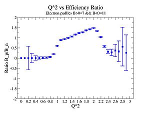 The ratio of inclusive electrons detected in scintillator paddle #7 when Btorus >0 (B_p)to inclusive electrons detected by paddle 11 when B<0(B_n) |
The inclusive missing mass W for each torus setting. Dashed line is B>0 and solid line is B<0 |
Media:electronefficiencyratioBp7Bn11.txt
Now plot efficiency as function of X_{BJ} and W < 1232 and require pion.
Positive Pion Efficiency dependence on [math]x_bj[/math]
Pion and electron both required.
W<1232 and [math]Q^2=1.1 GeV^2[/math]
Now cut on Q^2 where the inclusive electron rates are the same with both torus settings and then require at least one positive pion.
| X_bj |
B_n/B_p Rates
|
| 0.14 |
0.25 [math]\pm[/math] 0.55
|
| 0.15 |
0.74 [math]\pm[/math] 0.27
|
| 0.17 |
1.07 [math]\pm[/math] 0.18
|
| 0.19 |
1.3 [math]\pm[/math] 0.13
|
| 0.2 |
1.4 [math]\pm[/math] 0.14
|
There appears to be a region around X_{Bj}= 0.2 which has the same number of pions detected for both torus settings.
Negative Pion Efficiency dependence on [math]Q^2[/math]
Pion and electron both required(e_sector=7 for B>0 && e_sector=11 for B<11).
Now cut on Q^2 where the inclusive electron rates are the same with both torus settings and then require at least one positive pion.
| [math]Q^2[/math] |
B_p/B_n Rates
|
| 0.2 |
0.004 [math]\pm[/math]0.55
|
| 0.3 |
0.017 [math]\pm[/math] 0.5
|
| 0.4 |
0.069[math]\pm[/math] 0.6
|
| 0.5 |
0.0262[math]\pm[/math] 0.6
|
| 0.6 |
0.039[math]\pm[/math] 0.5
|
| 0.7 |
0.1 [math]\pm[/math]0.64
|
| 0.8 |
0.055[math]\pm[/math] 0.52
|
| 0.9 |
0.259[math]\pm[/math] 0.52
|
| 1 |
1.232[math]\pm[/math] 0.52
|
| 1.1 |
3.96[math]\pm[/math] 0.8
|
There DOES NOT appears to be a region which has the same number of negative pions detected for both torus settings.
What is wrong?
8/13/10
1.) Change Osipenko cuts to maximize electrons when B <0 but still minimize impact of negative pion contamination. Look at effects on Npe distribution.
Insert current number of electron events that are removed by the Osipenko cut for B<0. Compare it to event removed by other cuts.
2.) Schedule Prelim exam.
Shropshire has replaced cole.
Members are: Forest, Fisher, Shropshire, Dale, Tatar(?)
Ask Dustin McNulty
1.) [1]
"Original cut parameters generated by Osipenko et.al. were not very efficient for especially outbending data of eg1b experiment. The loss of electrons was substantial. For inbending data, loss of electrons were at acceptable level. To gain some electrons back we generated new cut parametes that will specifically work better for outbending data. Also we slightly adjusted the cut parameters for inbending data for some sectors and segments."
2.) Upgraded Proposal defense presentation(includes event display) File:TamarProposalP 1.pdf
11/10/10
DTS files used for analysis.
Media:ND3Bn.txt
Media:ND3Bp.txt
Media:NH3Bn.txt
Media:NH3Bp.txt
positive

negative
What are the cuts for the above histogram?
pion, OSI, EC
11/30/10
DST ntuple suggestions
- Event number and run number should be recorded. Run number is in RUNINFO. Event number should be in the event packet.
- Create variable called helicity and fill it with absolute helicity.
GEM detector
- order mylar and copper tape., 1" wide, $20 worth of each
- check DPO 4104 see if working properly
- find 10 frames for Qweak GEM foils (or order more)
- check gas supply
12/6/10
DST ntuple
Run number looks good.
PbPt values are all non-zero now.
1) Some of the TORUS values are zero when they should be positive?
Doesnt matter. There are totally four files: ND3_target+Torus_positive, ND3_target+Torus_negative, NH3_target+Torus_positive and NH3_target+Torus_negative. So not an issue.
2.) Electrons have less than 0.25 GeV energy?
Still dont know.
3.) ASYM=HWP*LINAC*P_T is in the root file.
4.) Where are the FC normalization histograms
Delta_D_over_D
12/20/10
DST
1.)
Looks like a particle ID problem for outbending (B<0) negative pions.
Calculate the missing mass for the and stor it in M_X. (included and corrected in NTUPLE)
Redo all the ntuples.
All ntuples are done.
2.) is run 27048 OK (no target run(empty)), corrected for both target runs
3.) Current quarks(the core of the constituent quark without the gluons and sea quarks(covering). The mass of the current quarks(up and down) is 5-10 MeV), light cone?
pion momentum for different torus settings and targets
pion paddle number for different torus settings
Need a before and after cuts histogram with stats to see number of events dropped
1/24/11
1.) Find energy range with substantial ND3, pi- events when B <0.
Ratio plot for Q^2 and X_{BJ}
once you find the Q^2 and X_BJ range holding a reasonable amount of data.
2.) Inclusive electron scattering ratio of
| Inclusiveelectrons -vs- Q-squared |
Inclusive Missing Mass (W) for 1.0 Q^2 <1.2
|
| [[|300px|thumb|The ratio of inclusive electrons detected in scintillator paddle #7 when Btorus >0 (B_p)to inclusive electrons detected by paddle 11 when B<0(B_n) NH3 Target]] |
[[|300px|thumb|The inclusive missing mass W for each torus setting. Dashed line is B>0 and solid line is B<0]]
|
| [[|300px|thumb|The ratio of inclusive electrons detected in scintillator paddle #7 when Btorus >0 (B_p)to inclusive electrons detected by paddle 11 when B<0(B_n)]]ND3 Target |
[[|300px|thumb|The inclusive missing mass W for each torus setting. Dashed line is B>0 and solid line is B<0]]
|
| [[|300px|thumb|The ratio of inclusive electrons detected in scintillator paddle #7 when Btorus >0 (B_p)to inclusive electrons detected by paddle 11 when B<0(B_n)]] Both Targets |
300px|thumb|The inclusive missing mass W for each torus setting. Dashed line is B>0 and solid line is B<0
|
3.) Semi Inclusive pion production ratios -vs- Q^2, Only electron cuts
/cache/mss/clas/eg1b/production/pass1/v4/4p2out/misc/dst/dst2828*
ND3 4.2-
28287
28288
28289
28311
28312
28313
28314
28315
28316
28317
28319
28320
28321
28322
28323
28335
28336
28337
28338
28339
28340
28341
28351
28352
28367
28368
28369
28370
28371
28372
28373
28374
28375
28376
28377
28378
28379
28380
28381
28385
28386
28389
28390
28391
28392
28393
28394
28396
28397
28398
28399
28400
28401
ND3 4.2+
28074
28075
28076
28077
28078
28079
NH3 4.2-
28407
28408
28409
28410
28411
28412
28413
28414
28415
28416
28417
28422
28423
28424
28425
28426
28427
28428
28429
28432
28433
28438
28439
28443
28445
28446
28447
28448
28449
28450
28456
28457
28458
28460
28461
28462
28463
28464
28467
28469
28471
28472
28473
28476
28478
28479
NH3 4.2+
28205
28207
28208
28209
28210
28211
28212
28214
28215
28216
28217
28222
28223
28224
28225
28226
28227
28230
28231
28232
28233
28234
28235
28236
28240
28242
28244
28245
28246
28247
28249
28250
28252
28253
28254
28255
28256
28260
28261
28262
28263
28264
28265
28266
28272
28274
28275
28276
28277
File locations http://www.jlab.org/Hall-B/secure/eg1/EG2000/nevzat/UPGRADE_DST/
/cache/mss/home/nguler/dst
Rates before and after requiring pions
all the cuts are applied, except NPHE>2.5 cut.
4.2 GeV, ND3 target, 98 files, B<0[math]\frac{\mbox{SemiInclusive Events}}{\mbox{Inclusive Events}}= 14.5% [/math]
4.2 GeV, ND3 target, 32 files, B>0[math]\frac{\mbox{SemiInclusive Events}}{\mbox{Inclusive Events}}= 4.4 %[/math]
The ratio for ND3 4.2 GeV data
Electron paddle selection
Inclusive
 |
|
| Electron Paddle Number(Inclusive, B<0, 4.2 GeV Beam, ND3 Target) |
Electron Paddle Number(Inclusive, B>0, 4.2 GeV Beam, ND3 Target)
|
Semi-Inclusive
 |
|
| Electron Paddle Number(Semi-Inclusive, B<0, 4.2 GeV Beam, ND3 Target) |
Electron Paddle Number(Semi-Inclusive, B>0, 4.2 GeV Beam, ND3 Target)
|
B>0, ND3 Electron paddle number=5
B<0, ND3 Electron paddle number=10
The Ratio
| X_B |
[math]\frac{ND3,Epaddle=5,B\gt 0}{ND3,Epaddle=10,B\lt 0}[/math] without pions |
[math]\frac{ND3,Epaddle=5,B\gt 0}{ND3,Epaddle=10,B\lt 0}[/math] with pions
|
| 0.3 |
[math]1.01 \pm 0.02[/math] |
[math] 1.2 \pm 0.1[/math]
|
| 0.35 |
[math]1.06 \pm 0.01[/math] |
[math]1.1 \pm 0.06[/math]
|
| 0.4 |
[math]1.1 \pm 0.01[/math] |
[math]1.03 \pm 0.08[/math]
|
| 0.45 |
[math]1.1 \pm 0.01[/math] |
[math]1.1 \pm 0.09[/math]
|
| 0.5 |
[math]0.9 \pm 0.02[/math] |
[math]0.6 \pm 0.2[/math]
|
| 0.55 |
[math]0.23 \pm 0.06[/math] |
[math]0.13 \pm 0.5[/math]
|
The ratio for NH3 4.2 GeV data
Electron paddle selection
Inclusive
 |
|
| Electron Paddle Number(Inclusive, B<0, NH3 target, 4.2 GeV Beam) |
Electron Paddle Number(Inclusive, B>0, NH3 target, 4.2 GeV Beam)
|
Semi-Inclusive
 |
|
| Electron Paddle Number(Semi-Inclusive, B<0, NH3 target, 4.2 GeV Beam) |
Electron Paddle Number(Semi-Inclusive, B>0, NH3 target, 4.2 GeV Beam)
|
B>0, NH3 Electron paddle number=5
B<0, NH3 Electron paddle number=10
The Ratio
| X_B |
[math]\frac{NH3,Epaddle=5,B\gt 0}{NH3,Epaddle=10,B\lt 0}[/math] without pions |
[math]\frac{NH3,Epaddle=5,B\gt 0}{NH3,Epaddle=10,B\lt 0}[/math] with pions
|
| 0.3 |
[math]1.02 \pm 0.01[/math] |
[math] 1.2 \pm 0.03[/math]
|
| 0.35 |
[math]1.08 \pm 0.008[/math] |
[math]1.01 \pm 0.02[/math]
|
| 0.4 |
[math]1.09 \pm 0.009[/math] |
[math]1.04 \pm 0.02[/math]
|
| 0.45 |
[math]1.19 \pm 0.01[/math] |
[math]1.1 \pm 0.03[/math]
|
| 0.5 |
[math]0.9 \pm 0.01[/math] |
[math]0.8 \pm 0.03[/math]
|
| 0.55 |
[math]0.2 \pm 0.03[/math] |
[math]0.18 \pm 0.09[/math]
|
1/31/11
Electron paddle number for B>0 is 5 and for B<0 - 10. The cut was applied on [math]X_B[/math] : [math]0.3\lt X_B\lt 0.6[/math]
Inclusive
1.) Overlap electron kinematic ([math]\theta[/math], W, Momentum) for B>0 and B<0 and ND3 and NH3.
(NH3,B>0), (NH3,B<0), (ND3,B>0) && (ND3,B<0)
 |
 |
|
| Electron Momentum((NH3,B>0), (NH3,B<0), (ND3,B>0) && (ND3,B<0)) |
Electron [math]\theta[/math] Angle((NH3,B>0), (NH3,B<0), (ND3,B>0) && (ND3,B<0)) |
W mass((NH3,B>0), (NH3,B<0), (ND3,B>0) && (ND3,B<0))
|
2.) Now plot ratio (B< 0/B>0) electron kinematic ([math]\theta[/math], W, Momentum) for ND3 and NH3. ( I expect 2 curves in one plot)
[math]\frac{ND3 B\lt 0}{ND3 B\gt 0}[/math], [math]\frac{NH3 B\lt 0}{NH3 B\gt 0}[/math]
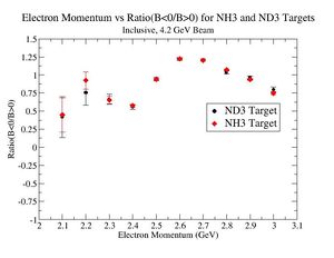 |
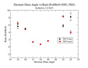 |
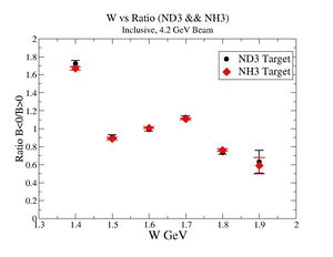
|
| Electron Momentum([math]\frac{ND3 B\lt 0}{ND3 B\gt 0}[/math], [math]\frac{NH3 B\lt 0}{NH3 B\gt 0}[/math]) |
Electron [math]\theta[/math] Angle([math]\frac{ND3 B\lt 0}{ND3 B\gt 0}[/math], [math]\frac{NH3 B\lt 0}{NH3 B\gt 0}[/math]) |
W mass([math]\frac{ND3 B\lt 0}{ND3 B\gt 0}[/math], [math]\frac{NH3 B\lt 0}{NH3 B\gt 0}[/math])
|
2.) Target ratio (B< 0/B>0) Difference electron kinematic ([math]\theta[/math], W, Momentum) (Ration for ND3 target - Ratio for NH3 target). ( I expect 1 curves in one plot)
[math]\frac{ND3 B\lt 0}{ND3 B\gt 0} - \frac{NH3 B\lt 0}{NH3 B\gt 0}[/math]
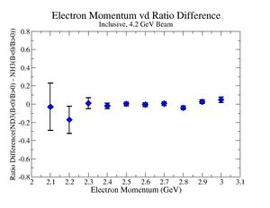 |
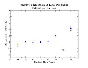 |
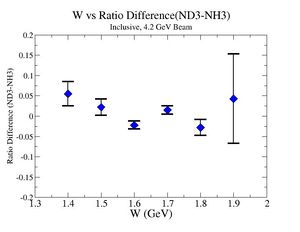
|
| Electron Momentum ([math]\frac{ND3 B\lt 0}{ND3 B\gt 0} - \frac{NH3 B\lt 0}{NH3 B\gt 0}[/math]) |
[math]\theta[/math] Theta Angle([math]\frac{ND3 B\lt 0}{ND3 B\gt 0} - \frac{NH3 B\lt 0}{NH3 B\gt 0}[/math]) |
W mass([math]\frac{ND3 B\lt 0}{ND3 B\gt 0} - \frac{NH3 B\lt 0}{NH3 B\gt 0}[/math])
|
Semi-Inclusive
(NH3,B>0), (NH3,B<0), (ND3,B>0) && (ND3,B<0)
 |
 |
|
| Electron Momentum((NH3,B>0), (NH3,B<0), (ND3,B>0) && (ND3,B<0)) |
Electron [math]\theta[/math] Angle((NH3,B>0), (NH3,B<0), (ND3,B>0) && (ND3,B<0)) |
W mass((NH3,B>0), (NH3,B<0), (ND3,B>0) && (ND3,B<0))
|
2


