Difference between revisions of "DeltaDoverD Progress"
| Line 702: | Line 702: | ||
<pre> | <pre> | ||
| − | What is on X-axis of FC | + | What is on X-axis of FC difference plots? It looks like the helicity |
| + | difference as a function of the number of FC counts. | ||
I would expect just 1 number representing a difference between | I would expect just 1 number representing a difference between | ||
the "+" heliciy FC counts and the "-" helicity FC counts. | the "+" heliciy FC counts and the "-" helicity FC counts. | ||
Revision as of 19:22, 6 June 2009
9/5/08
SIDIS Analysis
a.) Cross-Section comparison
i.) Calculate absolute cross section for = 0.5, 1 < Q^2 < 4 GeV^2 , W = 1.45 +/- 0.2 GeV
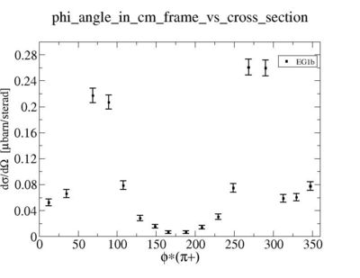
ii.) Plot -vs- when = -0.3 also plot -vs-
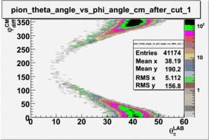
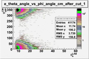
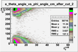
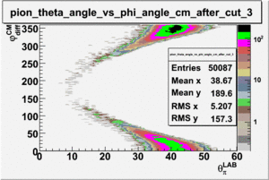
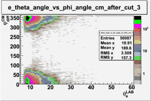
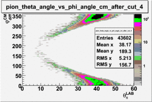
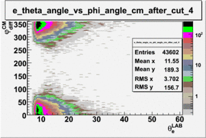
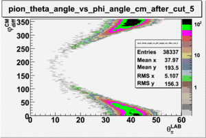
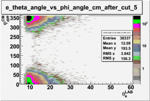
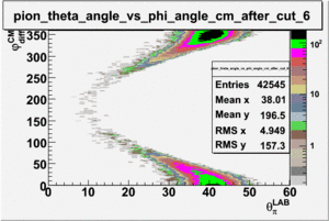
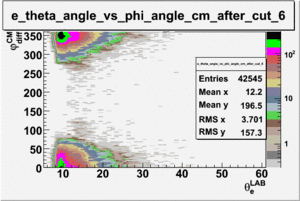
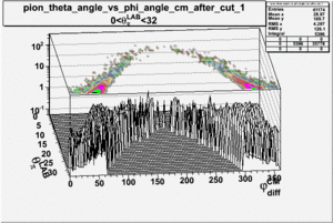
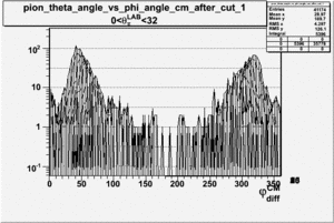
As one can see from histograms of the pion_theta_angle_vs_phi_angle_in_CM_Frame and the electron_theta_angle_vs_phi_angle_in_CM_Frame, the pion and electron acceptance in the region of is nearly zero(significantly low).
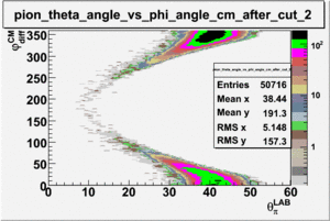
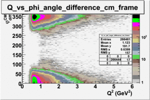
_vs_ plot shows that the cut should not make much difference on plot. The cut around should reduce the number of pions around 0 and 360 of phi angle.
9/19/08
SIDIS Analysis
a.) Cross-Section comparison
i.) Calculate absolute cross section for = 0.5, 1 < Q^2 < 4 GeV^2 , W = 1.45 +/- 0.2 GeV
?
- Documentation
The five-fold differential cross section for single pion production is equal to the following:
The Jacobian term can be given as:
where is the virtual photon flux and can be written as
The reason of having low cross section might be binning
In paper they use the following number of bins:
| Variable | Num. Bin | Range | Bin Size |
| W | 27 | 1.15 - 1.7 GeV | 20 MeV |
| 7 | 1.1 - 5.0 | variable | |
| 10 | -1.0 - 1.0 | 0.2 | |
| 24 | -180. - 180 | 15 |
Number of bins in my case were 360.
Number of bins equal is ~24
When i applied cut, the number of entries were reduced to 152.
In paper they use liquid-hydrogen unpolarized target(we have NH3 and ND3 polarized). The polarized electron beam current is 8 nA(in our case it is about 6 nA). and luminosity is different too. It also depends on statistics.
ii.) What is smallest angular coverage of EC (8 degrees?) Determine phi region where there is no acceptance ( where should we stop plotting data)?
iii.) Asymmetry Calculation
a.) Beam Asymmetry Plot
In order to plot Beam Asymmetry we need to plot for the first time the histogram of the invariant_mass_vs_cross_section. Then determine the structure function fitting the cross section and calculating the beam asymmetry function which is given as :
for given cos(theta) of the pion in cm, Q^2 and W invariant mass.
Choose kinematics ( a single theta and phi point )to max our stats and comparison to paper Histogram the following
- Number of e-pi coincidence events, number of FC counts
- Number of e-pi coincidence events/FC counts
- Number of e-pi coincidence events/FC count/Pt
for groups of runs with h_e,P_t = ++, +-, -+, --
table with 4 columns of h_e, P_t and 3 rows of the above histograms
9/26/08
SIDIS Analysis
1.) make semi-inclusive spectrum:
a.) h>0 Pt>0 b.) h > 0 pt<0 c.)h<0 pt>0 d.)h<0 pt<0
2.) ad up opposite target polarization histograms
3.) subtract h> 0 and h<0
helflag = 1 =>
helflag = 2 =>
helflag = 3 =>
helflag = 4 =>
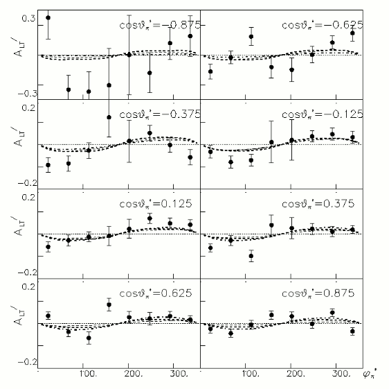
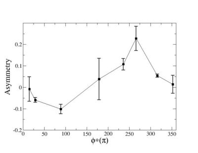
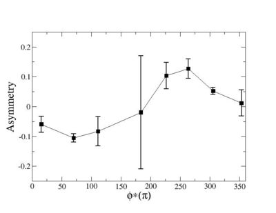
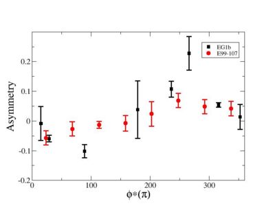
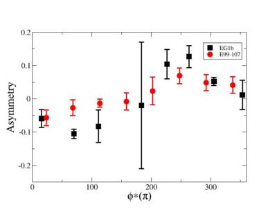
Phi_angle_CM vs Asymmetry
Compared data(there is no table for asymmetry values like cross section):
11/21/08
0.) insert run summarry table, Pb, Pt, PB*Pt, Btorus
1.) make semi-inclusive spectrum:
a.) h>0 Pt>0
b.) h > 0 pt<0
c.)h<0 pt>0
d.)h<0 pt<0
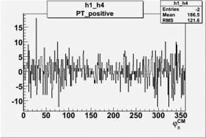
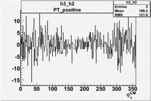
2.) helicity difference plots for Pt>0 and Pt<0
3.) Asym plots for Pt>0 and Pt< 0
4.) unpolarized target asymmetry
Rebin asymmetry hisograms and combine the two into a total asymmetry histogram
Run Summary Table
The table below should have run ranges with according to the elastic asymmetry measurements stored at http://www.jlab.org/Hall-B/secure/eg1/EG2000/eg1b_analysis_progress.htm.
http://www.jlab.org/Hall-B/secure/eg1/EG2000/josh/pbpt/
5.73 in
pos = 0.45743 +/- 0.04269
neg = -0.38816 +/- 0.04556
5.73 out
pos = 0.46604 +/- 0.03496
neg = -0.50684 +/- 0.03578
| Start Run Number | Beam Polarization(Pb) | Target Polarization(Pt) from dstdump file | Pb*Pt | Beam Torus | Beam Energy (MeV) |
| 26998 | 0 | -0.69 | 0.46604 | -2250 | 5736 |
| 26996 | -0.71 | -0.69 | 0.46604 | -2250 | 5736 |
| 26995 | -0.71 | -0.69 | 0.46604 | -2250 | 5736 |
| 26994 | -0.71 | -0.73 | 0.46604 | -2250 | 5736 |
| 26993 | -0.71 | -0.72 | 0.46604 | -2250 | 5736 |
| 26992 | -0.71 | -0.73 | 0.46604 | -2250 | 5736 |
| 26991 | -0.71 | -0.75 | 0.46604 | -2250 | 5736 |
| 26990 | -0.71 | -0.76 | 0.46604 | -2250 | 5736 |
| 26989 | 0.71 | -0.67 | -0.38816 | 2250 | 5736 |
| 26988 | 0.71 | -0.68 | -0.38816 | 2250 | 5736 |
| 26987 | 0.71 | -0.67 | -0.38816 | 2250 | 5736 |
| 26986 | 0.71 | -0.68 | -0.38816 | 2250 | 5736 |
| 26985 | 0.71 | -0.68 | -0.38816 | 2250 | 5736 |
| 26984 | 0.71 | -0.68 | -0.38816 | 2250 | 5736 |
| 26983 | 0.71 | -0.68 | -0.38816 | 2250 | 5736 |
| 26981 | 0.71 | -0.68 | -0.38816 | 2250 | 5736 |
| 26980 | 0.71 | -0.7 | -0.38816 | 2250 | 5736 |
| 26979 | 0.71 | -0.71 | -0.38816 | 2250 | 5736 |
| 26966 | 0.71 | 0.74 | 0.45743 | 2250 | 5736 |
| 26965 | 0.71 | 0.74 | 0.45743 | 2250 | 5736 |
| 26964 | 0.71 | 0.74 | 0.45743 | 2250 | 5736 |
| 26963 | 0.71 | 0.74 | 0.45743 | 2250 | 5736 |
| 26962 | 0.71 | 0.74 | 0.45743 | 2250 | 5736 |
| 26961 | 0.71 | 0.75 | 0.45743 | 2250 | 5736 |
| 26960 | 0.71 | 0.76 | 0.45743 | 2250 | 5736 |
| 26959 | 0.71 | 0.69 | 0.45743 | 2250 | 5736 |
| 26958 | 0.71 | 0.69 | 0.45743 | 2250 | 5736 |
| 26957 | 0.71 | 0.69 | 0.45743 | 2250 | 5736 |
| 26956 | 0.71 | 0.69 | 0.45743 | 2250 | 5736 |
| 26955 | 0.71 | 0.69 | 0.45743 | 2250 | 5736 |
| 26954 | 0.71 | 0.69 | 0.45743 | 2250 | 5736 |
| 26953 | 0.71 | 0.69 | 0.45743 | 2250 | 5736 |
| 26952 | 0.71 | 0.7 | 0.45743 | 2250 | 5736 |
| 26951 | 0.71 | 0.7 | 0.45743 | 2250 | 5736 |
| 26948 | 0.71 | 0.7 | 0.45743 | 2250 | 5736 |
| 26947 | 0.71 | 0.7 | 0.45743 | 2250 | 5736 |
| 26946 | 0.71 | 0.7 | 0.45743 | 2250 | 5736 |
| 26945 | 0.71 | 0.7 | 0.45743 | 2250 | 5736 |
| 26943 | 0.7 | 0.7 | 0.45743 | 2250 | 5736 |
| 26942 | 0.7 | 0.7 | 0.45743 | 2250 | 5736 |
| 26941 | 0.7 | 0.7 | 0.45743 | 2250 | 5736 |
| 26940 | 0.7 | 0.7 | 0.45743 | 2250 | 5736 |
| 26939 | 0.7 | 0.7 | 0.45743 | 2250 | 5736 |
| 26938 | 0.7 | 0.7 | 0.45743 | 2250 | 5736 |
| 26937 | 0.7 | 0.7 | 0.45743 | 2250 | 5736 |
| 26934 | 0.7 | 0.7 | 0.45743 | 2250 | 5736 |
| 26933 | 0.7 | 0.71 | 0.45743 | 2250 | 5736 |
| 26932 | 0.7 | 0.71 | 0.45743 | 2250 | 5736 |
| 26931 | 0.7 | 0.71 | 0.45743 | 2250 | 5736 |
| 26930 | 0.7 | 0.71 | 0.45743 | 2250 | 5736 |
| 26929 | 0.7 | 0.71 | 0.45743 | 2250 | 5736 |
| 26928 | 0.7 | 0.72 | 0.45743 | 2250 | 5736 |
| 26927 | 0.7 | 0.72 | 0.45743 | 2250 | 5736 |
| 26926 | 0.7 | 0.73 | 0.45743 | 2250 | 5736 |
| 26925 | 0.7 | 0.73 | 0.45743 | 2250 | 5736 |
| 27074 | 0.71 | -0.81 | -0.38816 | 2250 | 5736 |
| 27075 | 0.71 | -0.77 | -0.38816 | 2250 | 5736 |
| 27076 | 0.71 | -0.74 | -0.38816 | 2250 | 5736 |
| 27077 | 0.71 | -0.74 | -0.38816 | 2250 | 5736 |
| 27078 | 071 | -0.75 | -0.38816 | 2250 | 5736 |
| 27079 | 0.71 | -0.72 | -0.38816 | 2250 | 5736 |
| 27100 | 0.71 | 0.76 | 0.45743 | 2250 | 5736 |
| 27101 | 0.71 | 0.76 | 0.45743 | 2250 | 5736 |
| 27102 | 0.71 | 0.73 | 0.45743 | 2250 | 5736 |
| 27105 | 0.61 | 0.73 | 0.45743 | 2250 | 5736 |
| 27106 | 0.61 | 0.73 | 0.45743 | 2250 | 5736 |
| 27107 | 0.61 | -0.71 | -0.38816 | 2250 | 5736 |
| 27108 | 0.61 | -0.7 | -0.38816 | 2250 | 5736 |
| 27109 | 0.61 | -0.7 | -0.38816 | 2250 | 5736 |
| 27111 | 0.61 | -0.71 | -0.38816 | 2250 | 5736 |
| 27112 | 0.61 | -0.69 | -0.38816 | 2250 | 5736 |
| 27114 | 0.61 | 0 | 2250 | 5736 | |
| 27116 | -0.58 | 0.2 | -0.38816 | 2250 | 5736 |
| 27124 | -0.7 | 0.24 | -0.38816 | 2250 | 5736 |
| 27125 | -0.7 | 0.25 | -0.38816 | 2250 | 5736 |
| 27126 | -0.7 | 0.26 | -0.38816 | 2250 | 5736 |
| 27127 | -0.7 | 0.26 | -0.38816 | 2250 | 5736 |
| 27128 | -0.7 | 0.26 | -0.38816 | 2250 | 5736 |
| 27129 | -0.7 | 0.26 | -0.38816 | 2250 | 5736 |
| 27131 | -0.7 | 0.26 | -0.38816 | 2250 | 5736 |
| 27132 | -0.7 | 0.26 | -0.38816 | 2250 | 5736 |
| 27133 | -0.7 | 0.26 | -0.38816 | 2250 | 5736 |
| 27134 | -0.7 | 0.26 | -0.38816 | 2250 | 5736 |
| 27135 | -0.7 | 0.26 | -0.38816 | 2250 | 5736 |
| 27136 | -0.7 | 0.26 | -0.38816 | 2250 | 5736 |
| 27137 | -0.7 | 0.25 | -0.38816 | 2250 | 5736 |
| 27138 | -0.7 | 0.25 | -0.38816 | 2250 | 5736 |
| 27139 | -0.7 | 0.25 | -0.38816 | 2250 | 5736 |
| 27141 | -0.7 | 0.25 | -0.38816 | 2250 | 5736 |
| 27142 | -0.7 | 0.25 | -0.38816 | 2250 | 5736 |
| 27143 | -0.7 | 0.25 | -0.38816 | 2250 | 5736 |
| 27145 | -0.7 | 0.24 | -0.38816 | 2250 | 5736 |
| 27146 | -0.7 | 0.24 | -0.38816 | 2250 | 5736 |
| 27148 | -0.7 | 0.24 | -0.38816 | 2250 | 5736 |
| 27149 | -0.7 | -0.09 | 0.45743 | 2250 | 5736 |
| 27150 | -0.7 | -0.12 | 0.45743 | 2250 | 5736 |
| 27152 | -0.64 | -0.18 | 0.45743 | 2250 | 5736 |
| 27153 | -0.64 | -0.19 | 0.45743 | 2250 | 5736 |
| 27154 | -0.64 | -0.19 | 0.45743 | 2250 | 5736 |
| 27155 | -0.64 | -0.19 | 0.45743 | 2250 | 5736 |
| 27156 | -0.64 | -0.19 | 0.45743 | 2250 | 5736 |
| 27157 | -0.64 | -0.19 | 0.45743 | 2250 | 5736 |
| 27160 | -0.64 | -0.18 | 0.45743 | 2250 | 5736 |
| 27161 | -0.64 | -0.18 | 0.45743 | 2250 | 5736 |
| 27162 | -0.64 | -0.19 | 0.45743 | 2250 | 5736 |
| 27163 | -0.64 | -0.19 | 0.45743 | 2250 | 5736 |
| 27165 | -0.64 | -0.19 | 0.45743 | 2250 | 5736 |
| 27166 | -0.64 | 0.18 | -0.38816 | 2250 | 5736 |
| 27167 | -0.64 | 0.22 | -0.38816 | 2250 | 5736 |
| 27168 | -0.64 | 0.23 | -0.38816 | 2250 | 5736 |
| 27169 | -0.64 | 0.23 | -0.38816 | 2250 | 5736 |
| 27170 | -0.64 | 0.23 | -0.38816 | 2250 | 5736 |
| 27171 | -0.64 | 0.23 | -0.38816 | 2250 | 5736 |
| 27172 | -0.64 | -0.35 | 0.45743 | 2250 | 5736 |
| 27175 | -0.7 | -0.78 | 0.45743 | 2250 | 5736 |
| 27176 | -0.7 | -0.72 | 0.45743 | 2250 | 5736 |
| 27177 | -0.7 | -0.7 | 0.45743 | 2250 | 5736 |
| 27178 | -0.7 | -0.69 | 0.45743 | 2250 | 5736 |
| 27179 | -0.7 | -0.67 | 0.45743 | 2250 | 5736 |
| 27180 | -0.7 | -0.67 | 0.45743 | 2250 | 5736 |
| 27181 | -0.7 | -0.66 | 0.45743 | 2250 | 5736 |
| 27182 | -0.7 | -0.72 | 0.45743 | 2250 | 5736 |
| 27183 | -0.7 | -0.68 | 0.45743 | 2250 | 5736 |
| 27184 | -0.7 | -0.63 | 0.45743 | 2250 | 5736 |
| 27186 | -0.7 | 0.72 | -0.38816 | 2250 | 5736 |
| 27187 | -0.7 | 0.71 | -0.38816 | 2250 | 5736 |
| 27188 | -0.7 | 0.71 | -0.38816 | 2250 | 5736 |
| 27189 | -0.7 | 0.7 | -0.38816 | 2250 | 5736 |
| 27190 | -0.7 | 0.69 | -0.38816 | 2250 | 5736 |
| 27191 | -0.7 | 0.69 | -0.38816 | 2250 | 5736 |
| 27192 | -0.7 | 0.68 | -0.38816 | 2250 | 5736 |
| 27193 | -0.7 | 0.69 | -0.38816 | 2250 | 5736 |
| 27194 | -0.7 | 0.7 | -0.38816 | 2250 | 5736 |
| 27195 | -0.7 | 0.69 | -0.38816 | 2250 | 5736 |
| 27113 | 0.61 | 0.68 | 0.45743 | 2250 | 5736 |
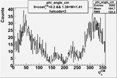
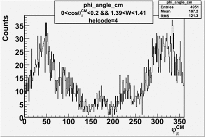
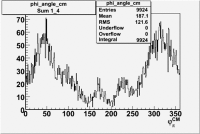
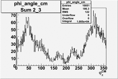
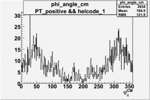
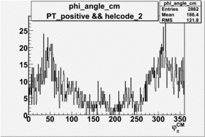
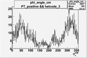
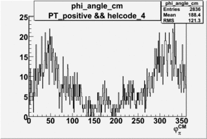
Phi_Angle_CM_Frame for Positive and Negative Target Polarization
| Helcode # | Negative Target Polarization | Positive Target Polarization |
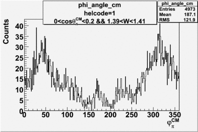
| 1 h>0 | 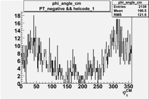 |
|
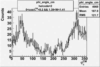
| 2 h<0 | 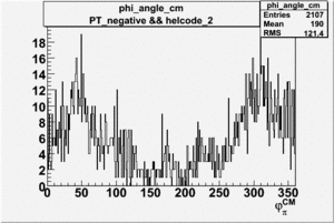 |
|
| 3 | 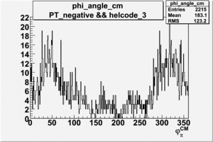 |
|
| 4 | 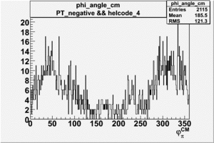 |
|
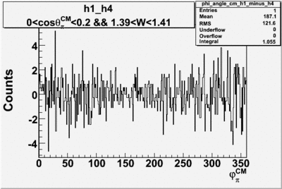
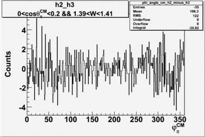
Helicity Difference Plots for Pt>0 and Pt<0
| Helicity Difference | Negative Target Polarization | Positive Target Polarization |
| h1-h4 | 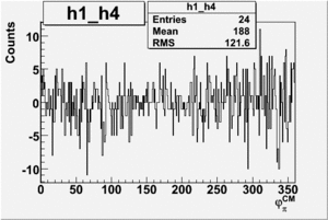 |
|
| h3-h2 | 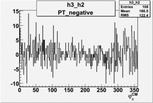 |
|
12/12/08
1.) Fix table of Pb Pt
2.) Asym plots for Pt>0, Pt< 0, combined
3.) unpolarized target asymmetry
Unpolarized Target Asymmetry
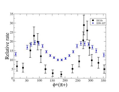
1.) Subtract and compare to beam asymemtry data from E99-107
5-01-2009
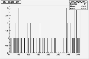
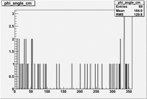
Target and Beam Polarization are positive
| Helcode # | Negative Beam Torus | Positive Beam Torus |
| 1 h>0 | 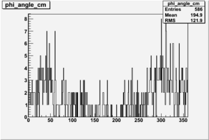 |
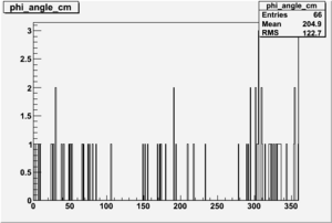
|
| 2 h<0 | 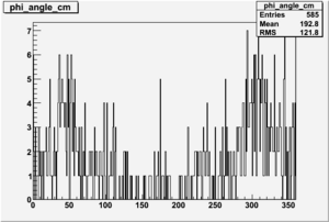 |
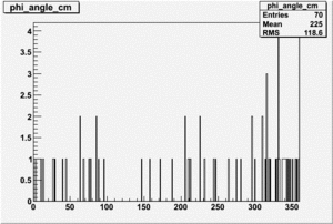
|
| 3 | 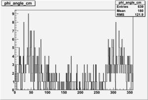 |
|
| 4 | 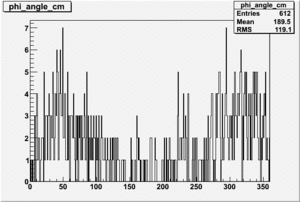 |
|
Target Polarization Positive and Beam Polarization Negative
| Helcode # | Negative Beam Torus | Positive Beam Torus |
| 1 h>0 | No Data | 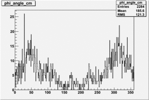
|
| 2 h<0 | No Data | 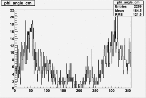
|
| 3 | No Data | 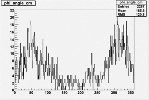
|
| 4 | No Data | 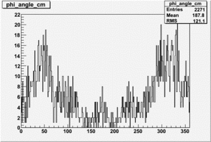
|
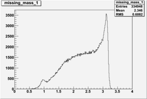
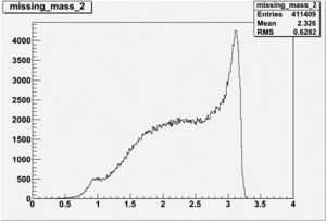
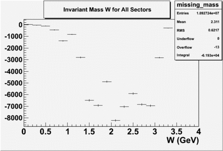
Inclusive Histograms For Invariant Mass
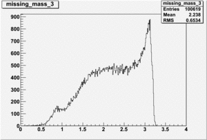
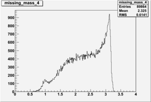
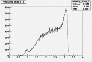
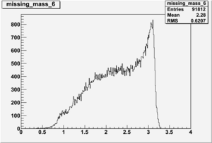
Invariant Mass Histograms for Each Sector
All helicities
Helcode=1
300px300px
300px300px
300px300px
3/20/09
1.) plot Wdiff
2.) plot PE using Osipenko/Josh cuts
05/27/09
| Run Number | W vs | |
| 26991 | 100px |  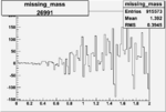 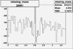
|
| 26990 | 100px | 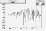 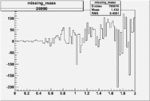 
|
| 26989 | 150px |   
|
| 26988 | 150px |   
|
| 26987 | 150px |   
|
| 26986 | 150px |   
|
| 26985 | 150px |   
|
| 26983 | 150px | 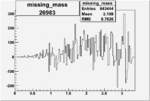 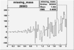 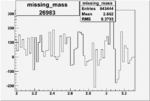
|
| 26965 | 150px | 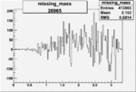  
|
| 26964 | 150px |   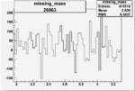
|
| 26961 | 150px | 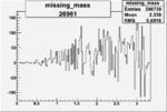 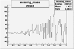 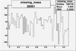
|
| 26959 | 150px | 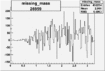 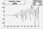 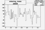
|
| 26958 | 150px | 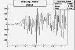 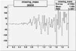 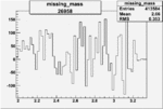
|
| 26956 | 150px | 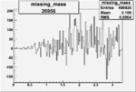 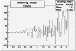 
|
| 26955 | 150px |   
|
| 26954 | 150px | 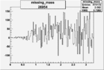 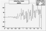 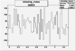
|
| 26952 | 150px | 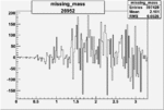 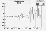 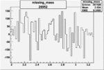
|
| 26947 | 150px | 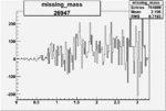 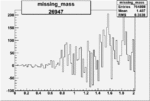 
|
| 26945 | 150px |   
|
| 26943 | 150px |   
|
| 26942 | 150px |  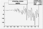 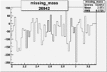
|
| 26941 | 150px | 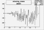 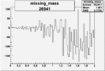 
|
| 26940 | 150px |   
|
| 26939 | 150px |   
|
| 26938 | 150px |   
|
| 26937 | 150px |   
|
| 26934 | 150px |   
|
| 26933 | 150px | 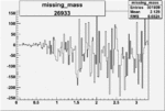 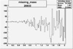 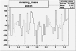
|
06/6/09
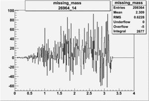
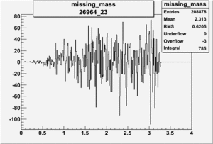
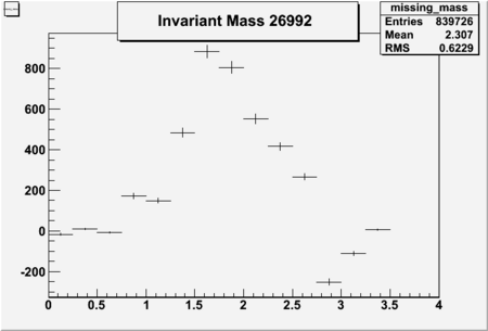
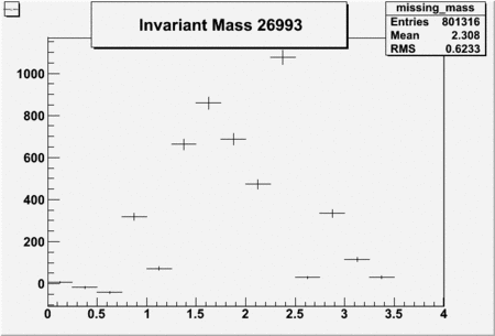
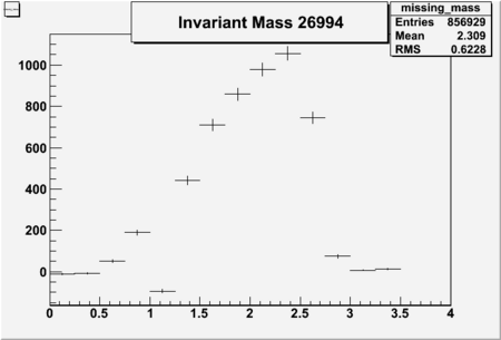
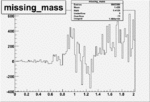
Invariant Mass
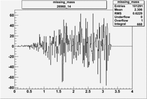
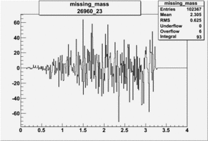
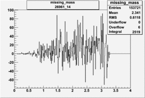
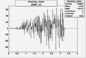
Difference of Invariant Mass for two differnet cuts:
| Run Number | EC Cuts+ requiring pion | OSI Cuts | EC Cuts | |
| 26991 |  |
 |
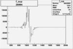
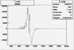
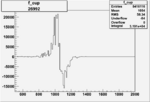
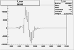
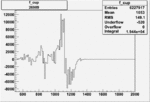
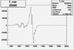
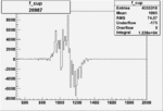
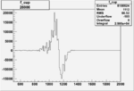
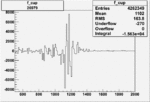
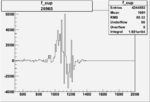
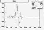
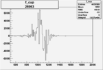
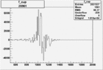
What is on X-axis of FC difference plots? It looks like the helicity
difference as a function of the number of FC counts.
I would expect just 1 number representing a difference between
the "+" heliciy FC counts and the "-" helicity FC counts.
Another way to calculate the FC asymmetry is on a pulse pair basis.
A pulse pair is an "original" and a "complement" helicity state.
You histogram the FC asymmetry for each pair.  While this is a good measure
of the FC asymmetry, in practice we normalize the W spectrum over an entire run/file.
| Run Number | W difference | FC difference | |
| 26991 |  |
150px | |
| 26994 | 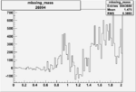 |
 |
|
| 26993 | 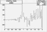 |
 |
|
| 26992 | 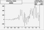 |
 |
|
| 26990 | 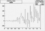 |
 |
|
| 26989 | 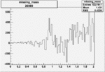 |
 |
|
| 26988 | 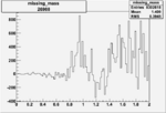 |
 |
|
| 26987 | 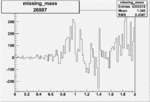 |
 |
|
| 26986 | 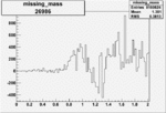 |
 |
|
| 26979 | 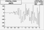 |
 |
|
| 26965 | 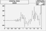 |
 |
|
| 26964 | 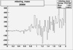 |
 |
|
| 26963 | 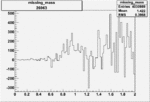 |
 |
|
| 26961 | 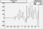 |
 |
NPHE
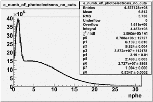
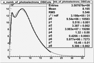
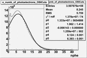
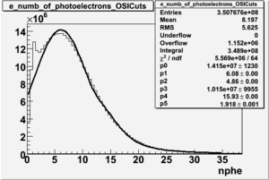
To find out pion contamination in the electron sample i used Osipenko geometrical cuts. The number of photoelectrons before and after osipenko cuts are shown below:
| No cuts | OSI Cuts |
For different fits:
- Conclusions
