Calculating kinematic variables in Moller Lab Frame
Vector Magnitude
The pythagorean theorem is used to take the 3 cartesean components in the Lab frame to find the magnitude of the Moller momentum vector, [math]|\vec{p}_2\ '|[/math].
[math]|\vec{p}_2\ '|=\sqrt{p_x^2+p_y^2+p_z^2}[/math]
Finding the correct kinematic values starting from knowing the momentum of the Moller electron, [math]p^'_{2}[/math] , in the Lab frame,
xz Plane
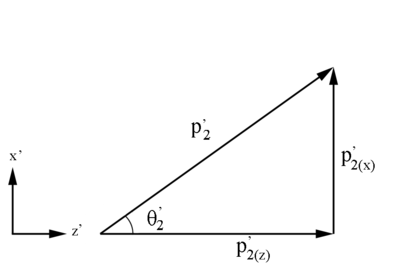 Figure 1: Definition of Moller electron variables in the Lab Frame in the x-z plane.
Using [math]\theta '_2=\arccos \left(\frac{p^'_{2(z)}}{p^'_{2}}\right)[/math]
| [math]\Longrightarrow {p^'_{2(z)}=p^'_{2}\cos(\theta '_2)}[/math]
|
Checking on the sign resulting from the cosine function, we are limited to:
| [math]0^\circ \le \theta '_2 \le 60^\circ \equiv 0 \le \theta '_2 \le 1.046\ Radians[/math]
|
Since,
[math]\frac{p^'_{2(z)}}{p^'_{2}}=cos(\theta '_2)[/math]
[math]\Longrightarrow p^'_{2(z)}\ should\ always\ be\ positive[/math]
xy Plane
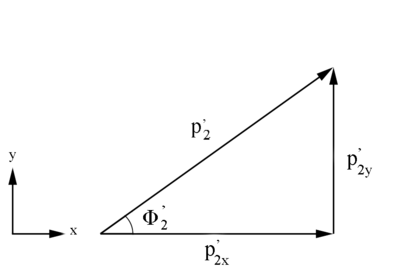 Figure 2: Definition of Moller electron variables in the Lab Frame in the x-y plane.
Similarly, [math]\phi '_2=\arccos \left( \frac{p^'_{2(x) Lab}}{p^'_{2(xy)}} \right)[/math]
where [math]p_{2(xy)}^'=\sqrt{(p_{2(x)}^')^2+(p^'_{2(y)})^2}[/math]
[math](p^'_{2(xy)})^2=(p^'_{2(x)})^2+(p^'_{2(y)})^2[/math]
and using [math]p^2=p_{(x)}^2+p_{(y)}^2+p_{(z)}^2[/math]
this gives [math](p^'_{2})^2=(p^'_{2(xy)})^2+(p^'_{2(z)})^2[/math]
[math]\Longrightarrow (p'_{2})^2-(p'_{2(z)})^2 = (p'_{2(xy)})^2[/math]
[math]\Longrightarrow p_{2(xy)}^'=\sqrt{(p^'_{2})^2-(p^'_{2(z)})^2}[/math]
which gives[math]\phi '_2 = \arccos \left( \frac{p_{2(x)}'}{\sqrt{p_{2}^{'\ 2}-p_{2(z)}^{'\ 2}}}\right)[/math]
| [math]\Longrightarrow p_{2(x)}'=\sqrt{p_{2}^{'\ 2}-p_{2(z)}^{'\ 2}} \cos(\phi)[/math]
|
Similarly, using [math]p_{2}^2=p_{2(x)}^2+p_{2(y)}^2+p_{2(z)}^2[/math]
[math]\Longrightarrow p_{2}^{'\ 2}-p_{2(x)}^{'\ 2}-p_{2(z)}^{'\ 2}=p_{2(y)}^{'\ 2}[/math]
| [math]p_{2(y)}'=\sqrt{p_{2}^{'\ 2}-p_{2(x)}^{'\ 2}-p_{2(z)}^{'\ 2}}[/math]
|
[math]p_{x}[/math] and [math]p_{y}[/math] results based on [math]\phi[/math]
Checking on the sign from the cosine results for [math]\phi '_2[/math]
We have the limiting range that [math]\phi[/math] must fall within:
| [math]-\pi \le \phi '_2 \le \pi\ Radians[/math]
|
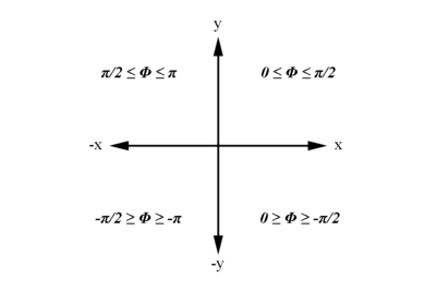
Examining the signs of the components which make up the angle [math]\phi[/math] in the 4 quadrants which make up the xy plane:
| [math]For\ 0 \ge \phi '_2 \ge \frac{-\pi}{2}\ Radians[/math]
|
| px=POSITIVE
|
| py=NEGATIVE
|
| [math]For\ 0 \le \phi '_2 \le \frac{\pi}{2}\ Radians[/math]
|
| px=POSITIVE
|
| py=POSITIVE
|
| [math]For\ \frac{-\pi}{2} \ge \phi '_2 \ge -\pi\ Radians[/math]
|
| px=NEGATIVE
|
| py=NEGATIVE
|
| [math]For\ \frac{\pi}{2} \le \phi '_2 \le \pi\ Radians[/math]
|
| px=NEGATIVE
|
| py=POSITIVE
|
Analysis.groovy
From a GEMC run of solenoid field strength of 0T, the eg12_rec.0.evio output file of the reconstruction is analyzed. The different kinematic variables are displayed as shown:
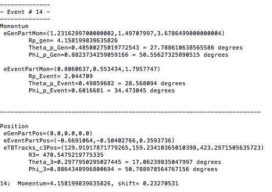
Using the phythagorean theorm to construct the Generated Event momentum vector length, we find:
[math]|\vec{p}_2\ '|=\sqrt{1.23162997^2+1.49707997^2+3.6786499^2}=4.15819983964[/math]
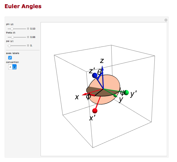
Euler Angles
We can use the Euler angles to perform the rotations.
For the rotation about the y axis.
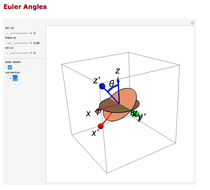
And the rotation about the z axis.
Transformation Matrix
The Euler angles can be applied using a transformation matrix
[math]\left(
\begin{array}{ccc}
\cos (\theta ) & 0 & -\sin (\theta ) \\
0 & 1 & 0 \\
\sin (\theta ) & 0 & \cos (\theta ) \\
\end{array}
\right).\left(
\begin{array}{c}
x \\
y \\
z \\
\end{array}
\right)[/math][math]=\left(
\begin{array}{c}
x \cos (\theta )-z \sin (\theta ) \\
y \\
z \cos (\theta )+x \sin (\theta ) \\
\end{array}
\right)[/math]
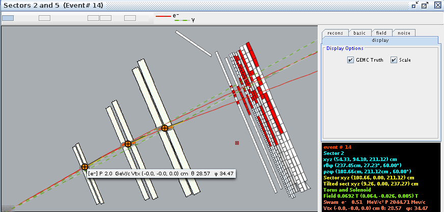
For event #29, in sector 3, the location of the first interaction is given by
Converting -25 degrees to radians,
[math]\theta =-0.436332[/math]
which is the rotation the detectors are rotated from the y axis.
[math]\left(
\begin{array}{ccc}
\cos (\theta ) & 0 & -\sin (\theta ) \\
0 & 1 & 0 \\
\sin (\theta ) & 0 & \cos (\theta ) \\
\end{array}
\right).\left(
\begin{array}{c}
-15.76 \\
0 \\
237.43 \\
\end{array}
\right)[/math][math]=\left(
\begin{array}{c}
86.0588 \\
0. \\
221.845 \\
\end{array}
\right)[/math]
Finding [math]\phi =\frac{120\ 2 \pi }{360};[/math] since "sector -1" =3-1=2*60=120 degrees
[math]\left(
\begin{array}{ccc}
\cos (\phi ) & -\sin (\phi ) & 0 \\
\sin (\phi ) & \cos (\phi ) & 0 \\
0 & 0 & 1 \\
\end{array}
\right).\left(
\begin{array}{c}
86.0588 \\
0. \\
221.845 \\
\end{array}
\right)[/math][math]=\left(
\begin{array}{c}
-43.0294 \\
74.5291 \\
221.845 \\
\end{array}
\right)[/math]
This shows how the coordinates are transformed and explains the validity of using the TBTracking information to obtain a phi angle in the lab frame.


