Difference between revisions of "DC Binning Based On Wire Numbers"
(Created page with "The bin size based on wire number will need to be a uniform width of 1, as in an increment of 1 between the integer values of the wires. This uniformity in bin size based on wir…") |
|||
| (30 intermediate revisions by the same user not shown) | |||
| Line 1: | Line 1: | ||
| + | <center><math>\underline{\textbf{Navigation}}</math> | ||
| + | |||
| + | [[CED_Verification_of_DC_Angle_Theta_and_Wire_Correspondance|<math>\vartriangleleft </math>]] | ||
| + | [[VanWasshenova_Thesis#Determining_wire-theta_correspondence|<math>\triangle </math>]] | ||
| + | [[Detector_Geometry_Simulation|<math>\vartriangleright </math>]] | ||
| + | |||
| + | </center> | ||
| + | |||
| + | =DC Binning Based on Wire Numbers= | ||
| + | |||
The bin size based on wire number will need to be a uniform width of 1, as in an increment of 1 between the integer values of the wires. This uniformity in bin size based on wire numbers is not uniform when viewed by the angle theta due to the Drift Chamber geometry discussed earlier. | The bin size based on wire number will need to be a uniform width of 1, as in an increment of 1 between the integer values of the wires. This uniformity in bin size based on wire numbers is not uniform when viewed by the angle theta due to the Drift Chamber geometry discussed earlier. | ||
| − | Modifying | + | Modifying evio2root.cc |
| + | The corresponding theta scale can be superimposed over the bin plot using the minimum and maximum angles | ||
| − | |||
| − | <center> | + | <center><math>\theta_{n=1}=5.23^{\circ}\ \ \ \theta_{n=112}=41.07^{\circ}</math></center> |
| + | |||
| + | |||
| + | Since the scale on the axis describing the wire number bins runs from 0 to 113, we will account for these theoretical theta using the polynomial fit for the expression of theta as a function of the wire number. | ||
| + | |||
| + | <center><math>\theta_{n}=4.93253 +0.297371 n+0.000566298 n^2-3.04016 \times 10^{-6} n^3</math></center> | ||
| + | |||
| + | |||
| + | <center><math>\theta_{n=0}=4.93^{\circ}\ \ \ \theta_{n=113}=41.38^{\circ}</math></center> | ||
| + | |||
<pre> | <pre> | ||
gStyle->SetStripDecimals(kTRUE); | gStyle->SetStripDecimals(kTRUE); | ||
| − | TF1 *fit_function=new TF1("fit_function","[0]+[1]*x+[2]*x*x+[3]*x*x*x",4. | + | TF1 *fit_function=new TF1("fit_function","[0]+[1]*x+[2]*x*x+[3]*x*x*x",4.93,41.38); |
| − | fit_function->SetParameters(4. | + | fit_function->SetParameters(4.93253,0.297371,0.000566298,-.00000304016); |
TGaxis *A1 = new TGaxis(0,5000,113,5000,"fit_function",510,"-"); | TGaxis *A1 = new TGaxis(0,5000,113,5000,"fit_function",510,"-"); | ||
A1->SetTitle("Angle Theta(degrees)"); | A1->SetTitle("Angle Theta(degrees)"); | ||
| Line 18: | Line 37: | ||
| − | <center> | + | |
| + | <center><gallery widths=500px heights=400px> | ||
| + | File:Layer1bins.png|'''Figure 5.1.1:''' An Isotropic CM frame distribution of bin hits in the DC for superlayer 1, layer 1 | ||
| + | File:Layer1bins_Isotropic.png|'''Figure 5.1.2:''' An Isotropic lab frame distribution of bin hits in the DC for superlayer 1, layer 1. | ||
| + | </gallery></center> | ||
| + | |||
| + | |||
| + | |||
| + | |||
| + | |||
<center>[[File:Layer1binWeighted_Isotropic.png]][[File:MolThetaLabWeighted2.png]]</center> | <center>[[File:Layer1binWeighted_Isotropic.png]][[File:MolThetaLabWeighted2.png]]</center> | ||
| + | |||
| + | <center><gallery widths=500px heights=400px> | ||
| + | File:Layer1binWeighted.png|'''Figure 5.1.3:''' An Isotropic CM frame distribution of bin hits in the DC for superlayer 1, layer 1 | ||
| + | File:MolThetaLabWeighted.png|'''Figure 5.1.4:''' An Isotropic lab frame distribution of bin hits in the DC for superlayer 1, layer 1. | ||
| + | </gallery></center> | ||
| + | |||
| + | |||
| + | |||
| + | <center><gallery widths=500px heights=400px> | ||
| + | File:Layer1binWeighted_Isotropic.png|'''Figure 5.1.5:''' An Isotropic CM frame distribution of bin hits in the DC for superlayer 1, layer 1 | ||
| + | File:MolThetaLabWeighted2.png|'''Figure 5.1.6:''' An Isotropic lab frame distribution of bin hits in the DC for superlayer 1, layer 1. | ||
| + | </gallery></center> | ||
| + | |||
| + | |||
| + | |||
Using the expression for n in terms of Theta: | Using the expression for n in terms of Theta: | ||
| Line 31: | Line 74: | ||
| − | |||
| − | |||
| + | <center><gallery widths=500px heights=400px> | ||
| + | File:MolThetaWireWeighted.png|'''Figure 5.1.5:''' An Isotropic CM frame distribution of bin hits in the DC for superlayer 1, layer 1 | ||
| + | File:MolThetaWireWeightedIsotropic.png|'''Figure 5.1.6:''' An Isotropic lab frame distribution of bin hits in the DC for superlayer 1, layer 1. | ||
| + | </gallery></center> | ||
| + | |||
| + | |||
| + | <center><gallery widths=500px heights=400px> | ||
| + | File:MolThetaWireWeightedAdjusted.png|'''Figure 5.1.7:''' An Isotropic CM frame distribution of bin hits in the DC for superlayer 1, layer 1 | ||
| + | File:MolThetaWireWeightedAdjustedIsotropic.png|'''Figure 5.1.8:''' An Isotropic lab frame distribution of bin hits in the DC for superlayer 1, layer 1. | ||
| + | </gallery></center> | ||
| + | |||
| + | |||
| + | |||
| + | <center><gallery widths=500px heights=400px> | ||
| + | File:TheoryDCbinsWire.png|'''Figure 5.1.9:''' An Isotropic CM frame distribution of bin hits in the DC for superlayer 1, layer 1 | ||
| + | File:TheoryDCbinsWireIsotropic.png|'''Figure 5.1.10:''' An Isotropic lab frame distribution of bin hits in the DC for superlayer 1, layer 1. | ||
| + | </gallery></center> | ||
| + | |||
| + | |||
| + | |||
| + | ---- | ||
| + | |||
| + | |||
| + | <center><math>\underline{\textbf{Navigation}}</math> | ||
| + | |||
| + | [[CED_Verification_of_DC_Angle_Theta_and_Wire_Correspondance|<math>\vartriangleleft </math>]] | ||
| + | [[VanWasshenova_Thesis#Determining_wire-theta_correspondence|<math>\triangle </math>]] | ||
| + | [[Detector_Geometry_Simulation|<math>\vartriangleright </math>]] | ||
| − | + | </center> | |
Latest revision as of 20:14, 15 May 2018
DC Binning Based on Wire Numbers
The bin size based on wire number will need to be a uniform width of 1, as in an increment of 1 between the integer values of the wires. This uniformity in bin size based on wire numbers is not uniform when viewed by the angle theta due to the Drift Chamber geometry discussed earlier.
Modifying evio2root.cc
The corresponding theta scale can be superimposed over the bin plot using the minimum and maximum angles
Since the scale on the axis describing the wire number bins runs from 0 to 113, we will account for these theoretical theta using the polynomial fit for the expression of theta as a function of the wire number.
gStyle->SetStripDecimals(kTRUE);
TF1 *fit_function=new TF1("fit_function","[0]+[1]*x+[2]*x*x+[3]*x*x*x",4.93,41.38);
fit_function->SetParameters(4.93253,0.297371,0.000566298,-.00000304016);
TGaxis *A1 = new TGaxis(0,5000,113,5000,"fit_function",510,"-");
A1->SetTitle("Angle Theta(degrees)");
A1->Draw();
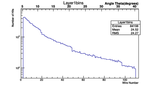
Figure 5.1.1: An Isotropic CM frame distribution of bin hits in the DC for superlayer 1, layer 1
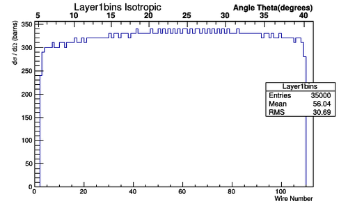
Figure 5.1.2: An Isotropic lab frame distribution of bin hits in the DC for superlayer 1, layer 1.


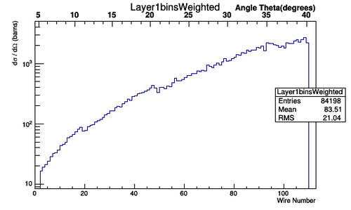
Figure 5.1.3: An Isotropic CM frame distribution of bin hits in the DC for superlayer 1, layer 1

Figure 5.1.4: An Isotropic lab frame distribution of bin hits in the DC for superlayer 1, layer 1.


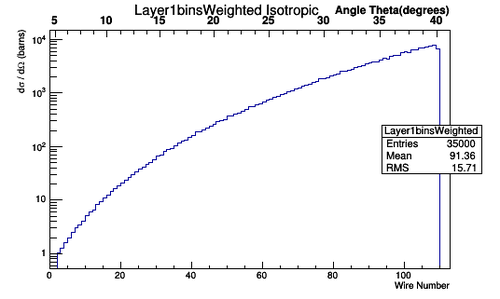
Figure 5.1.5: An Isotropic CM frame distribution of bin hits in the DC for superlayer 1, layer 1
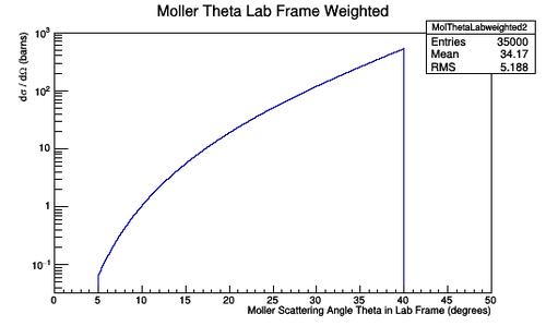
Figure 5.1.6: An Isotropic lab frame distribution of bin hits in the DC for superlayer 1, layer 1.
Using the expression for n in terms of Theta:
This relationship can be used to multiply each Moller Scattering angle theta in the lab frame, with it's differential cross-section weight, to find the Moller differential cross-section as a function of wire number in the lab frame.

Figure 5.1.5: An Isotropic CM frame distribution of bin hits in the DC for superlayer 1, layer 1
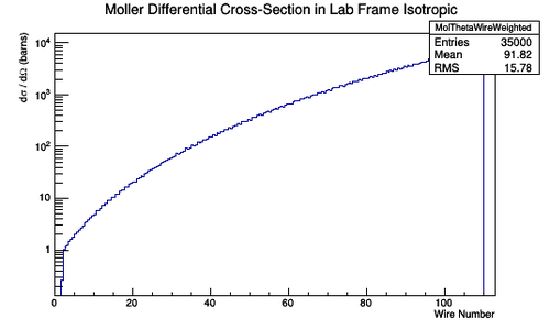
Figure 5.1.6: An Isotropic lab frame distribution of bin hits in the DC for superlayer 1, layer 1.


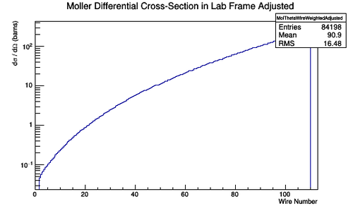
Figure 5.1.7: An Isotropic CM frame distribution of bin hits in the DC for superlayer 1, layer 1
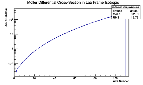
Figure 5.1.8: An Isotropic lab frame distribution of bin hits in the DC for superlayer 1, layer 1.


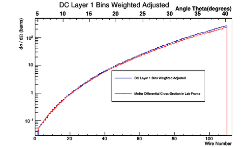
Figure 5.1.9: An Isotropic CM frame distribution of bin hits in the DC for superlayer 1, layer 1
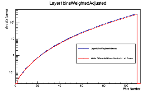
Figure 5.1.10: An Isotropic lab frame distribution of bin hits in the DC for superlayer 1, layer 1.

