Difference between revisions of "A W thesis"
| Line 528: | Line 528: | ||
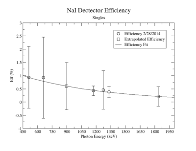
[[File:SingEffNaI.png | 400 px]] | [[File:SingEffNaI.png | 400 px]] | ||
| + | |||
| + | |||
| + | |||
| + | {| border="1" |cellpadding="20" cellspacing="0 | ||
| + | |- | ||
| + | | Run || Source || Energy || Expected rate (Hz) || NaI Det B Rate (ADC 7) (Hz) || NaI Eff (%) | ||
| + | |- | ||
| + | | 7027 || Na-22 ||511 || 1589.218 +/- 1.842 || 14.393 +/- 0.715 || 0.9057 +/- 1.2495 | ||
| + | |- | ||
| + | | 7025 || Cs-137 ||661.657 || 2548.03 +/- 0.222 || 22.8 +/- 0.9154 || 0.8948 +/- 1.520 | ||
| + | |- | ||
| + | | 7026 || Co-60 || 1173.228|| 1876.619 +/- 0.2687 || 7.529 +/- 0.5503 || 0.4012 +/- 0.3873 | ||
| + | |- | ||
| + | | 7027 || Na-22 || 1274.537|| 888.264 +/- 1.029 || 3.654 +/- 0.5266 || 0.4114 +/- 0.7940 | ||
| + | |- | ||
| + | | 7026 || Co-60 || 1332.492 || 1878.167 +/- 0.2690 || 6.784 +/- 0.5345 || 0.3612 +/- 0.3507 | ||
| + | |- | ||
| + | |} | ||
Revision as of 15:59, 2 October 2014
Introduction
Methods of determining atomic concentration in Material
Neutron Activation Analysis (NAA)
Neutron activation analysis (NAA) is a high-sensitivity and non-destructive multi-elemental analytical technique used for analysis of major, minor, and trace elements in samples. NAA is significantly different from other spectroscopic analytical techniques in that it is based on nuclear transitions rather than electronic transitions. The basic essentials to carry out an analysis of samples by NAA are a source of neutrons to bombard the sample, instruments suitable for detecting gamma rays, and knowledge of the reactions that occur when neutrons interact with target nuclei.
The sequence of events taking place during the most common type of nuclear reaction for NAA, namely neutron capture, is illustrated in the figure. (make figure) Upon irradiation, a neuron interacts with the target nucleus via a non-elastic collision. A compound nucleus forms in an excited and usually unstable state. This unfavourable state will almost instantaneously de-excite into a more stable configuration by emitting one or more characteristic prompt gamma rays. In most cases, this new and stable configuration yields a radioactive nucleus. The newly formed radioactive nucleus now decays by the emission of one of more characteristic delayed gamma rays. This decay process is at a much slower rate according to unique half-life of the radioactive nucleus. Measurement, in principle, falls into two categories: (1) prompt gamma-ray neutron activation analysis (PGNAA), where measurements are taken during the irradiation of a sample, or (2) the more common delayed gamma-ray neutron activation analysis (DGNAA), where measurements follow radioactive decay.
A range of different neutron sources can be used for NAA. These include reactors, accelerators, fusors, and radioisotopic neutron emitters. Since they have high fluxes of neutrons from uranium fission, nuclear reactors offer the highest available sensitivities for most elements.
There are several types of detectors and configurations employed in NAA. Most are designed to detect the emitted gamma radiation. The instrumentation most commonly used consists of scintillation type or semiconductor type detector(s), associated electronics, and a computer-based, multi-channel analyser. Scintillation type detectors use a radiation-sensitive crystal, usually thallium-doped sodium iodide (NaI(Tl)). Hyperpure or intrinsic germanium (HpGe) detectors that operate at liquid nitrogen temperatures (77 degrees K) are the semiconductor type most commonly operated for NAA.
There are a few drawbacks to the use of NAA. Even though the technique is non-destructive, the irradiated sample will remain radioactive for great lengths of time depending on the half-lives, requiring handling and disposal protocols. Also, not all labs have convenient access to a suitable reactor for a neutron source to irradiate a sample. As with any other analytical method, NAA is also not universal. For instance, the determination of low-Z elements, such as C, N, O, F, or several other elements such as Mg, Si, Ca, Ti, Ni, Sr, Y, Zr, Nb, Sn, and Tl, is not sufficiently sensitive or impossible.
Inductively coupled plasma mass spectrometry(ICP-MS)
Inductively coupled plasma atomic emission spectroscopy(ICP-OES)
Atomic Absorption Spectrometry (multi-element AAS)
Particle-induced X-ray Emission (PIXE)
Another method, uses X-ray from a synchrotron light source and look at the de-excitation of atomic electrons to measure the atomic number. Reports are that they can measure pico-gram quantities.
table of detection limits -vs- Method
Coincidence Counting Setup
Y-88 CAA
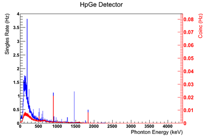
Using our Y-88 source, our set-up allows us to perform runs with the detectors in coincidence (AND mode) or singles (OR mode). The figure on the left shows the HpGe detector's coincidence events (red) that occurred within a 200 ns timing window. This graph has been overlaid with the same detector’s single events (blue). We can see that by having the detectors in coincidence, the noise is reduced and several peaks, which do not have multiple photons in coincidence, are removed.
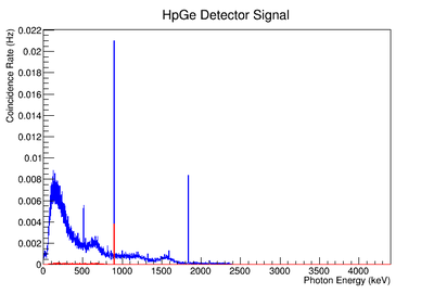
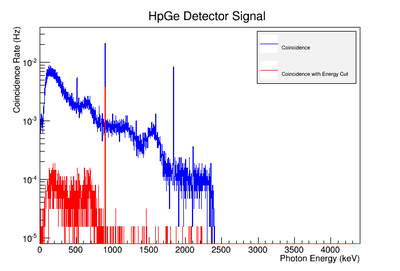
The coincidence run does not show the two energy peaks associated with Y-88 decay alone. Even though we require coincidence for the system to trigger, there is still noise. These peaks could be Compton events contaminating the coincidence and accidentals. Photons can loss a portion of their energy traveling to the detector. They do not necessarily have to deposit all of their energy into the detector either. The photon can Compton scatter out. It is not possible to tell the difference between a photon that deposited all of its energy from a scattered photon, since the speed of light is so fast and the resolution of the detector so poor. The photons can, however, be distinguished if an energy cut is applied. In order to remove the Compton events and the accidentals, we can require the photon energy to be completely deposited into the detector. This can be achieved by placing an energy cut on the NaI detector around the high energy Y-88 peak. This will remove other unwanted photon energies. The graph on the right is an overlay of the coincidence signal before (blue) and after (red) an energy cut is applied to the companion detector (NaI detector). The noise seen at low energies is greatly reduced after including the cut and improved the signal.
Background subtraction
898 keV analysis
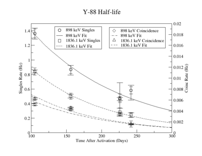
The raw Histograms and fits may be found here A_W_thesis_old#898_keV_signal_table
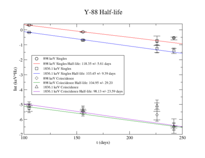
The Measured half life is
| Days | Trig | Integral | Statistical Error | Systematic Error | Systematic Error without Coincidence Energy Cut | |
| 105 | 0.98 | sing | 1.364 | N/A | ||
| coin | 0.0052 | |||||
| 156 | 1.46 | sing | 0.8697 | N/A | ||
| coin | 0.0042 | |||||
| 226 | 2.12 | sing | 0.4733 | N/A | ||
| coin | 0.0034 | |||||
| 242 | 2.27 | sing | 0.5807 | N/A | ||
| coin | 0.0015 |
The half-life with Ln y-axis:
The half-life with exponential fit:
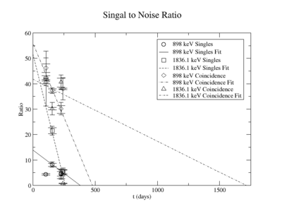
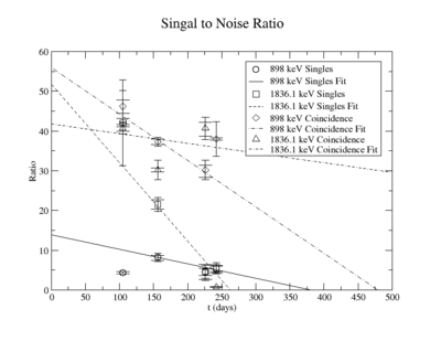
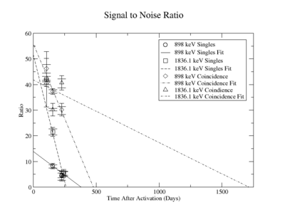
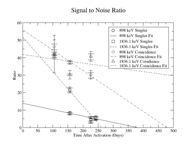
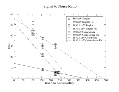
The signal to noise ratio is
| Days | Trig | SNR | Statistical Error | Systematic Error | |
| 105 | 0.98 | sing | 4.368 | ||
| coin | 46.181 | ||||
| 156 | 1.46 | sing | 8.228 | ||
| coin | 37.30 | ||||
| 226 | 2.12 | sing | 4.478 | ||
| coin | 30.195 | ||||
| 242 | 2.27 | sing | 5.494 | ||
| coin | 37.994 |
The first data point for the singles 898 keV was not included in the signal to noise fit. At the time of measurement, the noise was larger. This could be from contaminates with short half-lives in the sample that decayed away. Only elements with longer half-lives, such as Y-88, remained. The background of the remaining three data points were averaged.
For the 898 keV coincidence signal to noise fit, the last data point was not included. The length of the run and activities in the room, such as the nitrogen tank refilling, during counting caused the peak to be spread over a larger energy range. This also meant that the background noise would be larger. The background of the first three data points were averaged.
The following plots are of the signal to noise ratio with only the data points used to obtain a fit.
= 130.39 +/- 26.25 (s) and 108.18 +/- 0.4876 (c)
= 1.307e-8 (s) and 1.190e-11 (c)
= the time when SNR=0 using singles
= the time when SNR=0 using coinc
= 1.101e-9 = lowest measurable activity using singles
= 5.292e-13 = lowest measurable activity using coinc
=0.0879
=0.0085
1836.1 Analysis
The raw Histograms and fits may be found here A_W_thesis_old#1836_keV_signal_table
The Measured half life is
| Days | Trig | Integral | Statistical Error | Systematic Error | Systematic Error without Coincidence Energy Cut | |
| 105 | 0.98 | sing | 0.8414 | N/A | ||
| coin | 0.0062 | |||||
| 156 | 1.46 | sing | 0.5015 | N/A | ||
| coin | 0.0046 | |||||
| 226 | 2.12 | sing | 0.2822 | N/A | ||
| coin | 0.0062 | |||||
| 242 | 2.27 | sing | 0.2449 | N/A | ||
| coin | 0.0016 |
The half-life with Ln y-axis:
The half-life with exponential fit:
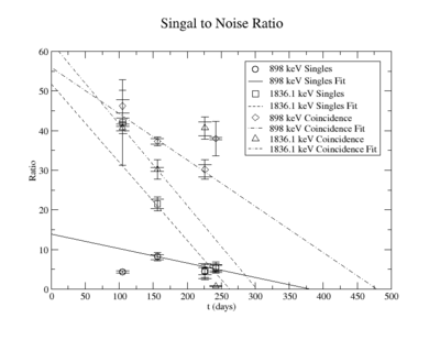
The signal to noise ratio is
| Days | Trig | SNR | Statistical Error | Systematic Error | |
| 105 | 0.98 | sing | 42.07 | ||
| coin | 40.666 | ||||
| 156 | 1.46 | sing | 21.52 | ||
| coin | 30.172 | ||||
| 226 | 2.12 | sing | 4.64 | ||
| coin | 40.666 | ||||
| 242 | 2.27 | sing | 5.43 | ||
| coin | 0.7569 |
For the 1836 keV coincidence signal to noise fit, the last data point was not included. The length of the run and activities in the room, such as the nitrogen tank refilling, during counting caused the peak to be spread over a larger energy range. This also meant that the background noise would be large. The background of the first three data points were averaged.
The following plots are of the signal to noise ratio with only the data points used to obtain a fit.
= 106.26 +/- 7.61 (s) and 100.10 +/- 4.0 (c)
= 1.786e-9 (s) and 1.509e-11 (c)
= the time when SNR=0 using singles
= the time when SNR=0 using coinc
= 3.253e-10 = lowest measurable activity using singles
= 2.174e-16 = lowest measurable activity using coinc
=0.0348
=2.75e-6
Error analysis
1.) rate energy cuts
2.) Energy calibration error
3.) Linear background fit error
4.) Gaussian integration of Signal - background peak
5.) ignorable error from run length time
6.) Coincidence energy cut.
7.) dividing by average background for SNR
8.) correction ratio for 3rd data point
9.) error in half life to find N0 for the detection limit extrapolation
10.) error extrapolation efficiency to higher energy lines for N0 calculation
Energy Window systematic error
The signal is measured by subtracting a count rate that is summed over an energy interval. The choice of this integration interval, energy window, is a source of systematic error. In order to calculate the error associated with the energy window, its range was adjusted based on the statistical variance of the background subtracted count rate fit to a gaussian. The integral was measured for window ranges chosen according to an integer interval of the standard deviation , where n = 3,4,5. The difference between the largest and mid-value was taken as the positive standard deviation, and the lowest was used for the standard deviation negative fluctuation. The resulting errors were divided by the signal to obtain a percent error as shown in column 1 of TableXXX.
Energy calibration systematic error
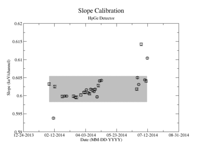
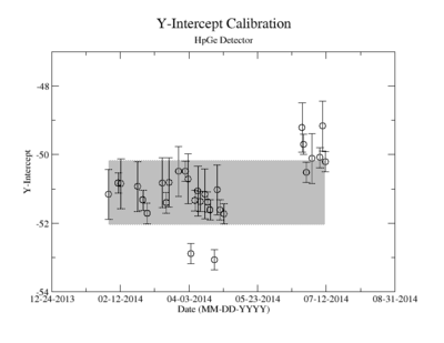
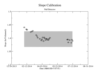
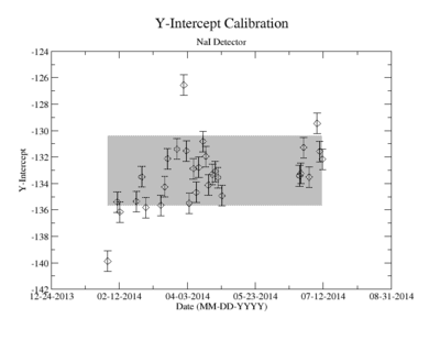
Prior to each measurement of the Y-88 sample's activity, the detectors where calibrated using several standard sources with known activity and dominant energy lines. This was accomplished by counting certified samples of Cs-137, Co-60, and Na-22 as well as Ba-133 and Mn-154. The observed mean ADC channel number was correlated with the expected energy line from each of the above sources. The correlation was measured using a standard linear fit algorithm. The linear fit algorithm determines the uncertainty of each fit parameter, the slope and the y-intercept. Figure YY.XX shows how the fit varies with time for the months take measure Y-88's half life. As shown in figure YY.XX, the fit's y-intercept has a temporal variance corresponding to an relative uncertainty of about 2%; the slope is about 0.5%. The effects of this error on the signals was analysed and is referred to as the energy calibration error. The range of the energy widow is held constant while the slope and the y-intercept where adjusted to account for all possible combinations with and without their respective error. The intergal value was recorded after every fit parameter change and the max, min, and mean values were obtained. The difference between the largest and mean value was taken as the positive standard deviation, and the lowest was used for the standard deviation's negative fluctuation. The resulting errors were divided by the signal to obtain a percent error as shown in column 2 of TableXXX.
Linear Fit Systematic error
The signal is determine by subtracting and underlying background. A estimate of this back is made by fitting the observed count rate with the function below :
.
The above function contains a Gaussian representing the measured signal and a linear function for the background. The linear fit parameters are used to create a histogram that is subtracted from the raw signal histogram, resulting in a histogram of just a signal. The energy window range used for the fit was adjusted and several fits performed to determine the uncertainty of the fit's slope and y-intercept. This systematic error, based on the fits dependence on the energy window is shown in the table under the column labeled "Linear Fit of Background". The fit parameters where adjusted to determine the maximum and minimum area of the background. For minimum background area, it was required that the area be positive. The difference between the maximum and unadjusted area value was taken as the positive standard deviation's fluctuation, and the minimum was used for the standard deviation's negative fluctuation. The resulting errors were divided by the signal to obtain a percent error as shown in column 3 of TableXXX.
Systematic error of the Coincidence Energy Cut
Half-life
898 keV Singles
| Days | Trig | Energy Window | Energy Calibration | Linear Fit of Background | Gaussian Integration of Signal | Total Systematic Error | |
| 105 | 0.98 | sing | |||||
| 156 | 1.46 | sing | |||||
| 226 | 2.12 | sing | |||||
| 242 | 2.27 | sing |
898 keV Coincidence
| Days | Trig | Energy Window | Energy Calibration | Linear Fit of Background | Gaussian Integration of Signal | Coincidence Energy | Total Systematic Error | Systematic Error without Coincidence Energy Cut | |
| 105 | 0.98 | coin | |||||||
| 156 | 1.46 | coin | |||||||
| 226 | 2.21 | coin | |||||||
| 242 | 2.27 | coin |
1836.1 keV Singles
| Days | Trig | Energy Window | Energy Calibration | Linear Fit of Background | Gaussian Integration of Signal | Total Systematic Error | |
| 105 | 0.98 | sing | |||||
| 156 | 1.46 | sing | |||||
| 226 | 2.12 | sing | |||||
| 242 | 2.27 | sing |
1836.1 keV Coincidence
| Days | Trig | Energy Window | Energy Calibration | Linear Fit of Background | Gaussian Integration of Signal | Coincidence Energy Cut | Total Systematic Error | Systematic Error without Coincidence Energy Cut | |
| 105 | 0.98 | coin | |||||||
| 156 | 1.46 | coin | |||||||
| 226 | 2.12 | coin | |||||||
| 242 | 2.27 | coin |
Signal to Noise Ratio
| Energy (keV) | Trig | Variance of Averaged Background |
| 898 | sing | |
| coin | ||
| 1836.1 | sing | N/A |
| coin |
The background's systematic error is being ignored.
898 keV Background
| Days | Trig | Background | Linear Fit of Background Error | Statistical Error | |
| 105 | 0.98 | sing | 0.3123 | N/A | |
| coin | 9.518e-5 | ||||
| 156 | 1.46 | sing | 0.0777 | ||
| coin | 8.732e-5 | ||||
| 226 | 2.12 | sing | 0.1532 | ||
| coin | 1.554e-4 | ||||
| 242 | 2.27 | sing | 0.0862 | ||
| coin | 3.948e-5 |
1836 keV Background
| Days | Trig | Background | Linear Fit of Background Error | Statistical Error | |
| 105 | 0.98 | coin | 1.037e-4 | ||
| 156 | 1.46 | coin | 4.248e-5 | ||
| 226 | 2.12 | coin | 3.112e-4 | ||
| 242 | 2.27 | coin | 2.114e-3 |
Efficiency
| Days | Trig | Extrapolation of Efficiency to High Energy | |
| 105 | 0.98 | sing | |
| coin | |||
| 156 | 1.46 | sing | |
| coin | |||
| 226 | 2.12 | sing | |
| coin | |||
| 242 | 2.27 | sing | |
| coin |
Detection Limit Extrapolation
| Days | Trig | Half-life Error to Find N0 | |
| 105 | 0.98 | sing | |
| coin | |||
| 156 | 1.46 | sing | |
| coin | |||
| 226 | 2.12 | sing | |
| coin | |||
| 242 | 2.27 | sing | |
| coin |
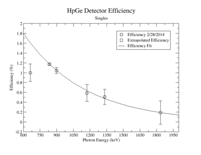
Singles Efficiency on 2/28/2014
HpGe Detector
| Run | Source | Energy | Expected rate (Hz) | HpGe Det B Rate (ADC 7) (Hz) | HpGe Eff (%) |
| 7027 | Na-22 | 511 | 1589.218 +/- 49.425 | 18.07 +/- 0.111 | 1.137 +/- 0.0317 |
| 7025 | Cs-137 | 661.657 | 2548.03 +/- 80.008 | 25.468+/- 0.172 | 0.9995 +/- 0.0321 |
| 7029 | Mn-54 | 834.848 | 41.405 +/- 1.300 | 0.485 +/- 0.014 | 1.171 +/- 0.0427 |
| 7026 | Co-60 | 1173.228 | 1876.619 +/- 58.926 | 11.03 +/- 0.106 | 0.588 +/- 0.0328 |
| 7027 | Na-22 | 1274.537 | 888.264 +/- 27.625 | 4.857 +/- 0.034 | 0.5468 +/- 0.0319 |
| 7026 | Co-60 | 1332.492 | 1878.167 +/- 58.974 | 9.584 +/- 0.023 | 0.510 +/- 0.0315 |
Extrapolated Efficiency
| Source | Energy | HpGe Eff (%) |
| Y-88 | 898 | 1.044 +/- 0.0618 |
| Y-88 | 1836.1 | 0.1909 +/- 0.237 |
NaI Detector
| Run | Source | Energy | Expected rate (Hz) | NaI Det B Rate (ADC 7) (Hz) | NaI Eff (%) |
| 7027 | Na-22 | 511 | 1589.218 +/- 49.425 | 14.86 +/- 0.0945 | 0.9351 +/- 0.0317 |
| 7025 | Cs-137 | 661.657 | 2548.03 +/- 80.008 | 23.45 +/- 0.9729 | 0.9203 +/- 0.0520 |
| 7026 | Co-60 | 1173.228 | 1876.619 +/- 58.926 | 8.001 +/- 0.0953 | 0.4264 +/- 0.0336 |
| 7027 | Na-22 | 1274.537 | 888.264 +/- 27.625 | 4.05 +/- 0.0247 | 0.4559 +/- 0.0317 |
| 7026 | Co-60 | 1332.492 | 1878.167 +/- 58.974 | 7.234 +/- 0.1675 | 0.3852 +/- 0.0390 |
| Run | Source | Energy | Expected rate (Hz) | NaI Det B Rate (ADC 7) (Hz) | NaI Eff (%) |
| 7027 | Na-22 | 511 | 1589.218 +/- 1.842 | 14.393 +/- 0.715 | 0.9057 +/- 1.2495 |
| 7025 | Cs-137 | 661.657 | 2548.03 +/- 0.222 | 22.8 +/- 0.9154 | 0.8948 +/- 1.520 |
| 7026 | Co-60 | 1173.228 | 1876.619 +/- 0.2687 | 7.529 +/- 0.5503 | 0.4012 +/- 0.3873 |
| 7027 | Na-22 | 1274.537 | 888.264 +/- 1.029 | 3.654 +/- 0.5266 | 0.4114 +/- 0.7940 |
| 7026 | Co-60 | 1332.492 | 1878.167 +/- 0.2690 | 6.784 +/- 0.5345 | 0.3612 +/- 0.3507 |
| Source | Energy | NaI Eff (%) |
| Y-88 | 898 | 0.5905 +/- 0.2423 |
| Y-88 | 1836.1 | 0.1925 +/- 0.3473 |
Coincidence Efficiency
| Source | HpGe Singles 898 keV Eff (%) | NaI Singles 1836.1 keV Eff (%) | HpGe Coincidence Eff (%) |
| Y-88 | 1.044 +/- 0.0618 | 0.2108 +/- 0.37 | 0.2201 +/- 0.387 |
Ba-133 CAA
Useful commands
Converting CODA data file to ROOT
make sure the CODA and ROOT environmental variables are setup by source the following scripts
source ~/CODA/setup
source ~/ROOT/root/bin/thisroot.csh
Now change to the data subdirectory and execute the program to convert the data file to root
cd /data
~/CODA/CODAreader/ROOT_V5.30/V785V792/evio2nt -fr6994.dat > /dev/null
rename the file so it has the .root extension allowing ROOT to identify it in the browser
mv r6994 r6994.root
Calibration work
ADC7 Average Slope = 0.601839 +/- 0.003662033
ADC7 Average Y-intercept = -51.1025 +/- 0.953309
ADC3 Average Slope = 1.39597 +/- 0.029539420
ADC3 Average Y-Intercept = -133.007 +/- 2.66636
System's intrinsic err
Plot calibration parameters as a function of time
determine the variance of the parameters using several (>20) fits
Impact of higher order fits
Plot
Variance comes from several fits,.
Compare uncertainty when fit is E-vs-Channe to Channel-vs-E
Probably should use %error for the weighting
Concentration measurement
A comparison of the measure concentrations using singles and coincidence counting
