Difference between revisions of "A W thesis"
| Line 136: | Line 136: | ||
| <math>T_{1/2}</math> || Trig || Signal || BackG Subtracted || colspan="5" | Fit Parameters || Signal Area || Noise Area || SNR | | <math>T_{1/2}</math> || Trig || Signal || BackG Subtracted || colspan="5" | Fit Parameters || Signal Area || Noise Area || SNR | ||
|- | |- | ||
| − | | rowspan="2" | .98 <math>T_{1/2}</math>|| sing || [[File:Run7022_Y88_898_rawsignal_fit.png | 100 px ]] || [[File:Run7022_Y88_898_signalsub_fit.png | 100 px ]] || <math>\mu=</math> 897.34 +/- 0.0938 || <math>\sigma=</math> 0.750375 || A= 1.015 || B= | + | | rowspan="2" | .98 <math>T_{1/2}</math>|| sing || [[File:Run7022_Y88_898_rawsignal_fit.png | 100 px ]] || [[File:Run7022_Y88_898_signalsub_fit.png | 100 px ]] || <math>\mu=</math> 897.34 +/- 0.0938 || <math>\sigma=</math> 0.750375 || A= 1.015 || B= -0.00000885816 || C= 0.0603580 || 0.9987 +/- 0.0199 || 0.2360 +/- 0.0524 || 4.23 |
|- | |- | ||
| − | | coin ||[[File:Run7023_Y88_898_rawsignal_fit.png | 100 px ]] || [[File:Run7023_Y88_898_signalsub_fit.png | 100 px ]] || <math>\mu=</math> 896.90 +/- 0.0064 || <math>\sigma=</math> 1.00907 || A= 0.0194163 || B= | + | | coin ||[[File:Run7023_Y88_898_rawsignal_fit.png | 100 px ]] || [[File:Run7023_Y88_898_signalsub_fit.png | 100 px ]] || <math>\mu=</math> 896.90 +/- 0.0064 || <math>\sigma=</math> 1.00907 || A= 0.0194163 || B= -0.00000235661 || C= 0.00291777 || 0.0191 +/- 0.00038 || 0.00325 +/- 0.4496 || 5.88 |
|} | |} | ||
Revision as of 19:01, 5 August 2014
Introduction
Methods of determining atomic concentration in Material
Neutron Activation Analysis (NAA)
Inductively coupled plasma mass spectrometry(ICP-MS)
Inductively coupled plasma atomic emission spectroscopy(ICP-OES)
Atomic Absorption Spectrometry (multi-element AAS)
Particle-induced X-ray Emission (PIXE)
Another method, uses X-ray from a synchrotron light source and look at the de-excitation of atomic electrons to measure the atomic number. Reports are that they can measure pico-gram quantities.
table of detection limits -vs- Method
Coincidence Counting Setup
Y-88 CAA
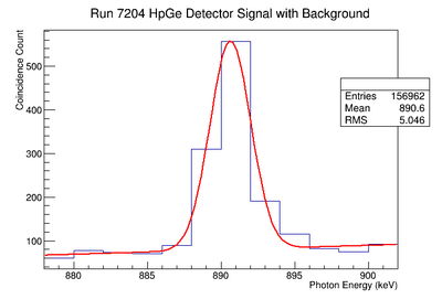
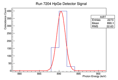
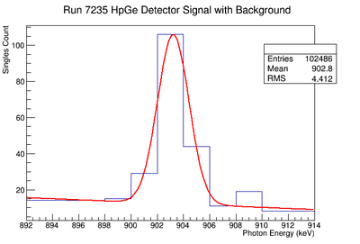
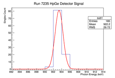
Background subtraction
Do the fit:
get parameters for line
Then fill 1 histogram with line
Then subtract
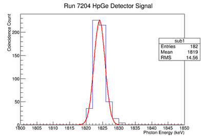
TH1F *coin1=new TH1F("coin1","coin1",30,1800,1860);

ntuple->Draw("ADC7*0.604963-49.7001 >>coin1")

TH1F *lin1=new TH1F("lin1","line1",30,1800,1860);

for(int i=1800;i<1861;i++){
lin1->Fill(i,-2028+1.12*i)
}

TH1F *sub1=new TH1F("sub1","sub1",30,1800,1860);

sub1->Add(coin1,1);
sub1->Add(lin1,-1);

sub1->Draw();
A pdf of the Mathematica notebook used to calculate background area, gaussian area, and plot signal/noise vs. activity.
Changed integration limits and re-fit r7235 File:AW Background Noise custom2.pdf
File:AW Background Noise custom3.pdf
All the ROOT fit parameters used to find the background and the resulting peaks. File:Y-88 Fit Log.pdf File:Y-88 Fit Log 2.pdf
Integrating the gaussian of the HpGe detector signal. File:AW Gaussian Integral.pdf
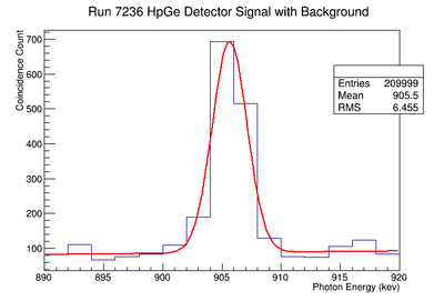
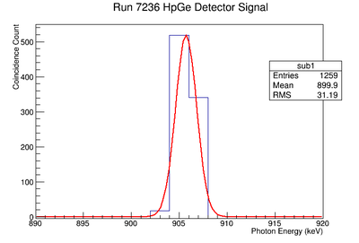
898 keV Signal and Background Noise Table
| Run # | Area of Signal | Area of Background | Signal to Noise Ratio |
| 7203 | 130.17 | 120.59 | 1.08 |
| 7204 | 825.34 | 558.66 | 1.48 |
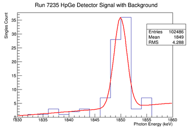
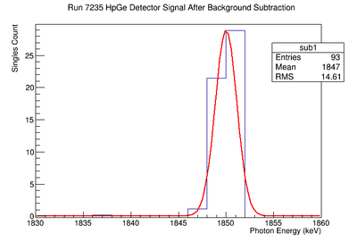
| 7235 | 194.38 | 60.23 | 3.23 |
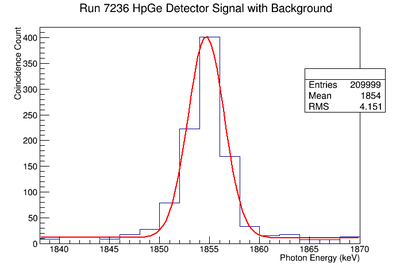
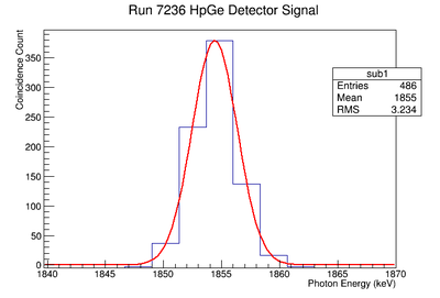
| 7236 | 1429.75 | 436.93 | 3.27 |
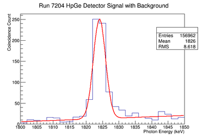
1836.1 keV Signal and Background Noise Table
| Run # | Area of Signal | Area of Background | Signal to Noise Ratio |
| 7203 | 83.29 | 24.73 | 3.37 |
| 7204 | 944.58 | 101.68 | 9.29 |
| 7235 | 82.25 | 20.90 | 3.94 |
| 7236 | 1849.86 | 97.64 | 18.95 |
Ba-133 CAA
Useful commands
Converting CODA data file to ROOT
make sure the CODA and ROOT environmental variables are setup by source the following scripts
source ~/CODA/setup
source ~/ROOT/root/bin/thisroot.csh
Now change to the data subdirectory and execute the program to convert the data file to root
cd /data
~/CODA/CODAreader/ROOT_V5.30/V785V792/evio2nt -fr6994.dat > /dev/null
rename the file so it has the .root extension allowing ROOT to identify it in the browser
mv r6994 r6994.root
Calibration work
System's intrinsic err
Plot calibration parameters as a function of time
determine the variance of the parameters using several (>20) fits
Impact of higher order fits
Plot
Variance comes from several fits,.
Compare uncertainty when fit is E-vs-Channe to Channel-vs-E
Probably should use %error for the weighting
Concentration measurement
A comparison of the measure concentrations using singles and coincidence counting
