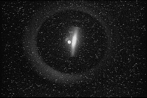
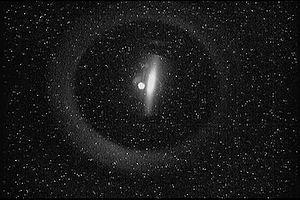
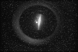
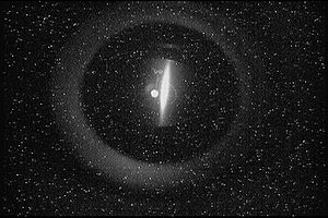
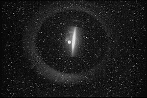
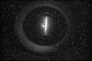
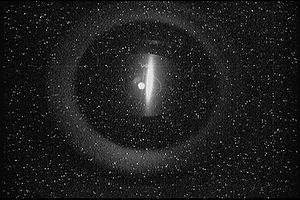
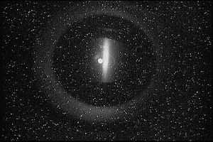
Difference between revisions of "Emittance Test"
| (166 intermediate revisions by 2 users not shown) | |||
| Line 16: | Line 16: | ||
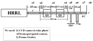
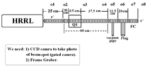
[[File:Emittance_Desien_27th_Jul_2010.png | 300 px]] | [[File:Emittance_Desien_27th_Jul_2010.png | 300 px]] | ||
| + | |||
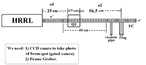
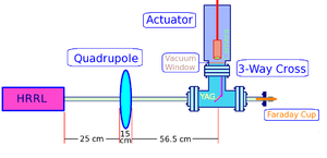
| + | [[File:HRRL_Emittance_Desien_27th_Jul_2010.png | 300 px]] | ||
Optim File on 27th, Jul. 2010: | Optim File on 27th, Jul. 2010: | ||
| Line 25: | Line 27: | ||
[[File:HRRL_Emittance.pdf]] | [[File:HRRL_Emittance.pdf]] | ||
| + | |||
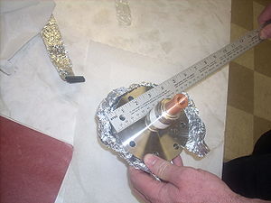
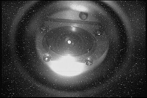
| + | == YAG (Yttrium Aluminum Garnet) Christal == | ||
| + | |||
| + | [[File:YAG_Christal_for_HRRL_2010_July_Emittance_Test.jpg | 300 px]] | ||
| + | |||
==Faraday Cup== | ==Faraday Cup== | ||
| Line 51: | Line 58: | ||
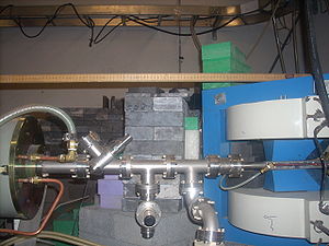
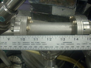
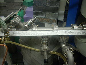
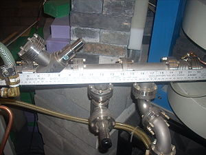
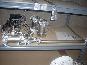
[[File:Beam_Line_Parts_HRRL_Positorns_2.jpg | 300 px]] | [[File:Beam_Line_Parts_HRRL_Positorns_2.jpg | 300 px]] | ||
[[File:Beam_Line_Parts_HRRL_Positorns_3.jpg | 300 px]] | [[File:Beam_Line_Parts_HRRL_Positorns_3.jpg | 300 px]] | ||
| − | |||
| − | |||
[[File:Beam_Line_Parts_HRRL_Positorns_6.jpg | 300 px]] | [[File:Beam_Line_Parts_HRRL_Positorns_6.jpg | 300 px]] | ||
[[File:Beam_Line_Parts_HRRL_Positorns_7.jpg | 300 px]] | [[File:Beam_Line_Parts_HRRL_Positorns_7.jpg | 300 px]] | ||
| Line 60: | Line 65: | ||
[[File:Beam_Line_Parts_HRRL_Positorns_11.jpg | 300 px]] | [[File:Beam_Line_Parts_HRRL_Positorns_11.jpg | 300 px]] | ||
[[File:Beam_Line_Parts_HRRL_Positorns_12.jpg | 300 px]] | [[File:Beam_Line_Parts_HRRL_Positorns_12.jpg | 300 px]] | ||
| + | |||
| + | |||
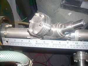
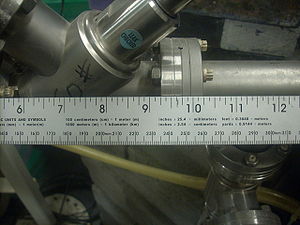
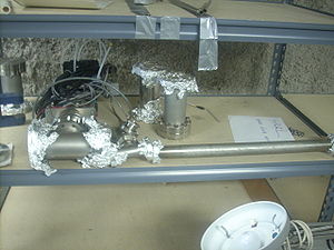
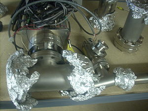
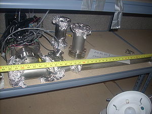
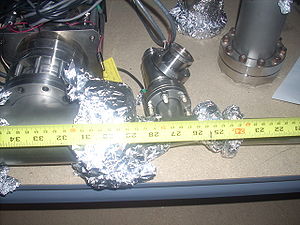
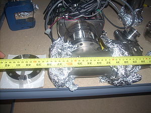
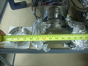
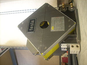
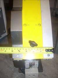
| + | Length of the pole face of Quad2Tin z direction is 8 cm. | ||
| + | |||
| + | [[File:Beam_Line_Parts_HRRL_Positorns_4.jpg | 300 px]] | ||
| + | [[File:Beam_Line_Parts_HRRL_Positorns_5.jpg | 200 px]] | ||
==Constructed Beam Line for Emittance Test == | ==Constructed Beam Line for Emittance Test == | ||
| Line 582: | Line 593: | ||
Root Code: [[File:Pixle.C]] | Root Code: [[File:Pixle.C]] | ||
| + | |||
| + | The cut is changed from circular to elliptical on Sep. 23rd, 2010. | ||
== Rotating the Image == | == Rotating the Image == | ||
| Line 1,077: | Line 1,090: | ||
|- | |- | ||
| || <math> 90.29 \pm 0.49 </math> || <math> 59.43 \pm 0.53 </math> || | | || <math> 90.29 \pm 0.49 </math> || <math> 59.43 \pm 0.53 </math> || | ||
| − | |||
| − | |||
| − | |||
| − | |||
|- | |- | ||
| || Horizontal mm/pixels || Vertical mm/pixels || | | || Horizontal mm/pixels || Vertical mm/pixels || | ||
|- | |- | ||
| − | | || <math> 0.1108 \pm 0.0006 </math> || <math> 0.1683 \pm 0.0015 </math> || | + | | || <math> 0.1108 \pm 0.0006 </math> || <math> 0.1683 \pm 0.0015 </math> || |
|- | |- | ||
|} | |} | ||
| Line 1,097: | Line 1,106: | ||
The fit is: | The fit is: | ||
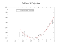
| − | <math> | + | <math> \sigma_x = (2.9098 \pm 0.0073) + (0.21775 \pm 0.00062)I + (0.006696 \pm 0.000047)I^{2} </math> |
| + | |||
| + | p-value is less than 0.000001 | ||
| + | |||
| + | For a parabola <math> y = a + bx + cx^{2} </math>, the <math> x </math> corresponding to the minimum <math> y_{min} </math> is: | ||
| + | |||
| + | <math> x_{min} = - \frac{b}{2c} </math>. | ||
| + | |||
| + | So, <math> I_{min} = -16.259707</math> | ||
| + | |||
| + | and | ||
| + | |||
| + | <math> \Delta I_{min} = \sqrt{ \frac{(\Delta b)^2}{4c^2} + \frac{ b^2 (\Delta c)^2}{4c^4} } </math>. | ||
| + | |||
| + | <math> \Delta I_{x,min} = \sqrt{ \frac{(0.00062)^2}{4 \times (0.006696)^2} + \frac{ (0.21775)^2 \times (0.000047)^2}{4 \times (0.006696)^4} } = 0.123161 | ||
| + | = 0.12</math>. | ||
| + | |||
| + | |||
| + | <math> I_{min} = -16.26 \pm 0.12 </math>. | ||
| + | |||
| + | |||
| + | <math> \sigma_{x,min} = 2.93671995816274 </math> | ||
| + | |||
| + | <math> \sigma_{x,min, up} = 2.94409703114234 </math> | ||
| + | |||
| + | <math> \sigma_{x,min, dn} = 2.92934288518313 </math> | ||
| + | |||
| + | |||
| + | <math> \sigma_{x,min,up} - \sigma_{x,min} = 0.007377072979601 </math> | ||
| + | |||
| + | <math> \sigma_{x,min} - \sigma_{x,min,dn}= 0.00737707297960144 </math> | ||
| + | |||
| + | |||
| − | + | So, | |
| + | <math> \sigma_{x,min} = 2.9367 \pm 0.0074 </math> | ||
==== Y Projection ==== | ==== Y Projection ==== | ||
| Line 1,108: | Line 1,150: | ||
The fit is: | The fit is: | ||
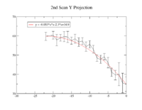
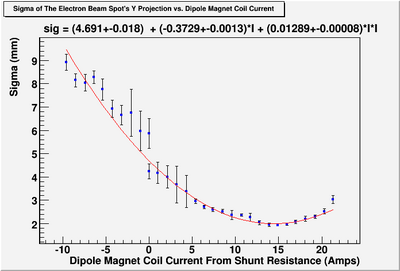
| − | <math> y = (4. | + | <math> \sigma_{y} = (4.691 \pm 0.018) + (-0.3729 \pm 0.0013)I + (0.01289 \pm 0.00008)I^{2} </math> |
| + | |||
| + | p-value is less than 0.000001 | ||
| + | |||
| + | <math> x_{min} = - \frac{b}{2c} </math>. | ||
| + | |||
| + | So, <math> I_{min} = 14.464701</math> | ||
| + | |||
| + | <math> \Delta I_{min} = \sqrt{ \frac{(\Delta b)^2}{4c^2} + \frac{ b^2 (\Delta c)^2}{4c^4} } </math>. | ||
| + | |||
| + | <math> \Delta I_{min} = \sqrt{ \frac{(0.0013)^2}{4 \times (0.01289) ^2} + \frac{ (-0.3729)^2 \times (0.00008)^2}{4 \times (0.01289)^4} } = 0.102966 </math> | ||
| + | |||
| + | |||
| + | <math> I_{min} = 14.46 \pm 0.10 </math>. | ||
| + | |||
| + | <math> \sigma_{y,min} = 4.65274050365148 </math> | ||
| + | |||
| + | <math> \sigma_{y,min, up} = 4.67087520809017 </math> | ||
| + | |||
| + | <math> \sigma_{y,min, dn} = 4.63487351175864 </math> | ||
| + | |||
| + | |||
| + | |||
| + | <math> \sigma_{y,min, up} - \sigma_{y,min} = 0.0181347044386939 </math> | ||
| + | |||
| + | <math> \sigma_{y,min} - \sigma_{y,min, dn}= 0.0178669918928378 </math> | ||
| + | |||
| + | |||
| + | |||
| + | So, | ||
| + | |||
| + | <math> \sigma_{y,min} = 4.653 \pm 0.018 </math> | ||
| + | |||
| + | |||
| + | ==== Conclusions ==== | ||
| + | |||
| + | |||
| + | For X projection: <math> I_{x,min} = -16.26 \pm 0.12</math>, and <math> \sigma_{x,min} = 2.9367 \pm 0.0074 </math> | ||
| + | |||
| + | |||
| + | For X projection: <math> I_{y,min} = 14.46 \pm 0.10 </math>, and <math> \sigma_{y,min} = 4.653 \pm 0.018 </math> | ||
| + | |||
| + | == Emittance == | ||
| + | |||
| + | Quadrupole Strength: <math> k = 0.2998 \frac{g[T/m]}{p[GeV]} </math> | ||
| + | |||
| + | g here is the gradient of the qudrupole. p is the momentum of the e- beam. | ||
| + | |||
| + | In our case, energy of the beam is 0.01 GeV and gap between dipole center and pole face is 1 inch. | ||
| + | |||
| + | <math> k = 0.2998 \frac{\frac{B(I)}{(1 inch)\times\frac{1 m}{1 inch}}[T/m]}{0.01 GeV} </math> | ||
| + | |||
| + | <math>B(I) = (3.6 \pm 1.3) \times 10^{-3} + (1945 \pm 2) \times 10^{-5} I [kG] = (3.6 \pm 1.3) \times 10^{-4} + (1945 \pm 2) \times 10^{-6} I [T] </math> | ||
| + | |||
| + | So, | ||
| + | |||
| + | <math> k = 0.2998 \frac{ (3.6 \pm 1.3) \times 10^{-4} + (1945 \pm 2) \times 10^{-6} I [T] }{0.01 \times 0.0254 [GeV][m]} </math> | ||
| + | |||
| + | <math> k = (0.42 \pm 0.16) + (2.2956 \pm 0.0024) \times I</math> | ||
| + | |||
| + | |||
| + | According to [[File:Emit_Meas_DAFNE_Linac_e_Beam.pdf]], for the case of quadruple scanning one quadrupole and screen, the emittance related to the quadrupole strength. | ||
| + | |||
| + | Transfer Matrix for 1uaruople \tilde{Q} and screen (drift space?) \tilde{S} consist the transfer matrix of the whole system as: | ||
| + | |||
| + | <math> \tilde{M} = \tilde{S}\tilde{Q} </math> | ||
| + | |||
| + | <math> \tilde{Q} = | ||
| + | \begin{bmatrix} | ||
| + | 1 & 0 \\ | ||
| + | k=\pm\frac{1}{f} & 1 | ||
| + | \end{bmatrix}. | ||
| + | </math> | ||
| + | |||
| + | <math> \tilde{S} = | ||
| + | \begin{bmatrix} | ||
| + | S_{11} & S_{12} \\ | ||
| + | S_{21} & S_{22} | ||
| + | \end{bmatrix}. | ||
| + | </math> | ||
| + | |||
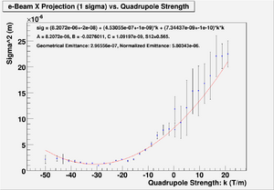
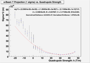
| + | <math> \sigma_{screen11} = Ak^2 - 2ABk + (C + AB^2) </math> | ||
| + | |||
| + | <math> \epsilon = \frac{\sqrt{AC}}{S^2_{12}} </math> | ||
| + | |||
| + | <math> S_{12} </math> is the distance between quadrupole and screen. | ||
| + | |||
| + | If I have a fit: | ||
| + | |||
| + | <math> \sigma_{screen11} = xk^2 + yk + z </math> | ||
| + | |||
| + | Then, <math> A=x, B=\frac{y}{-2A}, C=z-AB^2</math> | ||
| + | |||
| + | Two fits are: | ||
| + | |||
| + | [[File:Sigma_vs_QuadStrength_with_Fit_Projection_X.png | 300 px]] | ||
| + | |||
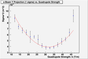
| + | [[File:Sigma_vs_QuadStrength_with_Fit_Projection_Y.png | 300 px]] | ||
| + | |||
| + | |||
| + | === Dr. Kim's Suggestion in his email === | ||
| + | |||
| + | from Yujong Kim <yjkim@isu.edu> | ||
| + | to Sadiq Setiniyaz <sadik82@gmail.com> | ||
| + | cc Dr Forest <tforest@athena.physics.isu.edu> | ||
| + | date Fri, Oct 8, 2010 at 6:44 AM | ||
| + | subject Re: Quad Scan Parameters | ||
| + | |||
| + | Dear Sadiq, | ||
| + | |||
| + | Many thanks, | ||
| + | |||
| + | I re-checked your QM scan fitting plot (final plots on emittance mewasurement). | ||
| + | |||
| + | Your fitting range too wide (-20 < k < 50). | ||
| + | |||
| + | Please fit again with a narrower range (+10 < k < 50). | ||
| + | Then, you can get much beautiful results. | ||
| + | Normally, we fit for only one k sign (positive or negative). | ||
| + | Yujong Kim | ||
| + | |||
| + | |||
| + | Here are results after doing Dr. Kim's suggested fit. | ||
| + | Note: I also corrected the distance S12 to the distance between quad center and screen (I originally did from the end of the quad to the screen, this is wrong). | ||
| + | |||
| + | ==== For X projection ==== | ||
| + | |||
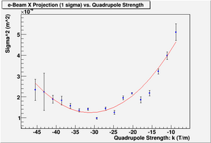
| + | [[File:HRRL_Emit_Parbola_Fit_Xaxis_as_BfieldStrength_DrKimSugFit.png | 300 px ]] | ||
| + | |||
| + | Minimum ChiSqrd is: 129.749 | ||
| + | |||
| + | The fit is: | ||
| + | |||
| + | sig^2 = (7.82463e-06+-2e-08) + (4.23945e-07+-1e-09)*k + (6.82167e-09+-1e-10)*k*k | ||
| + | |||
| + | Probability of obtaining data at least as incompatible with distribution as the data actually observed is 0.000000 | ||
| + | A = 7.82463e-06, B = -0.0270904, C = 1.07925e-09, S12=0.64. | ||
| + | Geometrical Emittance: 2.24354e-07 (m*rad), Normalized Emittance: 4.39048e-06 (m*rad). | ||
| + | |||
| + | |||
| + | Data file contains: Number-of-points B-Field-Strength Error-on-B-Field-Strength Sigma^2 Error-on-Sigma^2 | ||
| + | |||
| + | [[File:HRRL_Emit_Parbola_Fit_Xaxis_as_BfieldStrength.txt]] | ||
| + | |||
| + | |||
| + | |||
| + | ==== For Y projection ==== | ||
| + | |||
| + | [[File:HRRL_Emit_Parbola_Fit_Yaxis_as_BfieldStrength_DrKimSugFit.png | 300 px ]] | ||
| + | |||
| + | Minimum ChiSqrd is: 25.3174 | ||
| + | |||
| + | The fit is: | ||
| + | |||
| + | sig^2 = (1.71755e-05+-8e-08) + (-8.38108e-07+-3e-09)*k + (1.3229e-08+-1e-10)*k*k | ||
| + | |||
| + | Probability of obtaining data at least as incompatible with distribution as the data actually observed is 0.000000 | ||
| + | A = 1.71755e-05, B = 0.0243983, C = 3.00479e-09, S12=0.64. | ||
| + | Geometrical Emittance: 5.54629e-07 (m*rad), Normalized Emittance: 1.08538e-05 (m*rad). | ||
| + | |||
| + | Data file contains: Number-of-points B-Field-Strength Error-on-B-Field-Strength Sigma Error-on-Sigma | ||
| + | |||
| + | [[File:HRRL_Emit_Parbola_Fit_Yaxis_as_BfieldStrength.txt]] | ||
| + | |||
| + | === Data ROOTSYS Fit Script === | ||
| + | |||
| + | [[File:ROOTSCRIPT_for_HRRL_Emittace.C]] | ||
| + | |||
| + | ==Emittance Results for HRRL at 10 MeV and 102 micro Amp peak== | ||
| + | {| border="1" |cellpadding="20" cellspacing="0 | ||
| + | |- | ||
| + | | [[File:Emittance_HRRL_1mA.png | 500 px]] | ||
| + | |- | ||
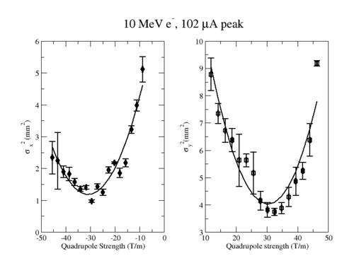
| + | |Measurements of the beam spot size as a function of the quadrupole magnetic field used to calculate the beam emittance. The fits are | ||
| + | <math>\sigma^2_x = (7.824\pm 0.02) + (0.424 \pm 0.001)k + (6.8 \pm 0.1 \times 10^{-9} )k^2</math> | ||
| + | and | ||
| + | <math>\sigma^2_y =17.17 \pm 0.08) - (0.084 \pm 0.003)k + (13.2 \pm 0.1e-10 \times 10^{-9}) k^2</math> with a<math> \chi^2/\nu</math> of 8.1 and 1.7 respectively. The respective P-values for this fit are 0.05 and 10^{-20}. | ||
| + | |} | ||
| + | |||
| + | [[File:Emmitance_HRRL_1mA_10-14-10.xmgrace.txt]] | ||
=Automatic Script to plot RMS= | =Automatic Script to plot RMS= | ||
| + | == ROOT == | ||
| + | |||
| + | How does the fit look when using the script below. | ||
| + | |||
| + | Working on it. | ||
| + | |||
| + | You should do background subtraction instead of cutting out the spot. | ||
| + | |||
| + | 2 bugs remain till Spe 24th. 1. entries; 2. Sub->Draw(); | ||
| + | |||
| + | Running Parabola_Fit_for_AutoRMS.C will run AutoRMS.C and do the fits. | ||
| + | |||
| + | |||
| + | [[File:AutoRMS.C]] | ||
| + | |||
| + | |||
| + | [[File:Parabola_Fit_for_AutoRMS.C]] | ||
| + | |||
| + | This 2 programs and pictures for data can be downloaded at: [http://inca.iac.isu.edu/~setiniyaz/All_Scan.tar.gz] | ||
| + | |||
| + | == MATLAB == | ||
| + | |||
| + | These MATLAB scripts will do Gaussian fits for beam spots and get rms beam size on x and projections (by Gauss_Fit.m). These rms values will be passed on (to Emit_Parabola_Fit_kl_YProjection.m and Emit_Parabola_Fit_kl_YProjection.m) to fit parabola. Parabola fit will be plotted,and emittances, normalized emittances, beta functions, alpha functions will given at the end. | ||
| + | |||
| + | [[File:Get_Emittance.rar]] | ||
| + | |||
| + | [[File:Guass_Fit.txt]] | ||
| + | |||
| + | [[File:Emit_Parabola_Fit_kl_XProjection.txt]] | ||
| + | |||
| + | [[File:Emit_Parabola_Fit_kl_YProjection.txt]] | ||
| + | |||
| + | [[File:gauss.txt]] | ||
| + | |||
| + | [[File:gausschisq.txt]] | ||
| + | |||
| + | [[File:gaussfit.txt]] | ||
| + | |||
| + | [[File:Plot_Beam_Spot.txt]] | ||
| + | |||
| + | [[File:Plot_Gauss_Fit.txt]] | ||
| + | |||
| + | [[File:ReadMe.txt]] | ||
| + | |||
| + | =Alternative Analysis from the East Cost= | ||
| + | |||
| + | [[Image Analysis]] | ||
| + | |||
| + | [[Emittance/TWISS parameter extraction]] | ||
| + | |||
| + | |||
| + | =New Fits with K1L= | ||
| + | |||
| + | == No Fringe Field Effect == | ||
| + | |||
| + | We want to do new fits with K1L. K1 is quadrupole strength and L is the thickness of the quadrupole. We will do it for the data we got previously. They are the following two data sets. | ||
| + | |||
| + | '''At this step, we will ignore fringe field effect, we want to consider it later.''' | ||
| + | |||
| + | |||
| + | need uncertainties in plots below | ||
| + | |||
| + | The uncertainties are difficult to believe because they are so small (< 0.1% !) | ||
| + | |||
| + | Redo you plots so they look like the ones below in terms of line boldness and quality. Identify the fit parameters and their error as well as a measurement of the goodness of fit. | ||
| + | |||
| + | https://wiki.iac.isu.edu/index.php/File:Emittance_HRRL_1mA.png | ||
| + | |||
| + | |||
| + | |||
| + | Data files contains: | ||
| + | |||
| + | Number-of-points B-Field-Strength Error-on-B-Field-Strength Sigma^2 Error-on-Sigma^2 | ||
| + | |||
| + | |||
| + | |||
| + | [[File:HRRL_Emit_Parbola_Fit_Xaxis_as_BfieldStrength.txt]] | ||
| + | |||
| + | [[File:HRRL_Emit_Parbola_Fit_Yaxis_as_BfieldStrength.txt]] | ||
| + | |||
| + | X-Projection: | ||
| + | Fit Parameters by MATLAB: | ||
| + | y = 0.00000784 + (0.00000288)*x + 0.00000031*x*x | ||
| + | Fit Parameters by Matrix Inversion: | ||
| + | y = (0.00000781+-0.00000027) + (0.00000282+-0.00000014)*x + (0.00000030+-0.00000002)*x*x | ||
| + | P-value = 7.6238e-21 | ||
| + | |||
| + | Y-Projection: | ||
| + | Fit Parameters by MATLAB: | ||
| + | y = 0.00001766 + (-0.00000599)*x + 0.00000066*x*x | ||
| + | Fit Parameters by Matrix Inversion: | ||
| + | y = (0.00001717+-0.00000084) + (-0.00000558+-0.00000041)*x + (0.00000059+-0.00000005)*x*x | ||
| + | P-value = 0.020964 | ||
| + | |||
| + | geometrical emittance: <math>\epsilon_{x} = 1.5 \pm 1.4 ~ mm*mrad</math> <math>\epsilon_{y} = 3.7 \pm 3.9 ~ mm*mrad </math> | ||
| + | normalized emittance: <math>\epsilon_{n,x} = 29 \pm 27 ~ mm*mrad</math> <math>\epsilon_{n,y} = 72.0 \pm 77.0 ~ mm*mrad </math> | ||
| + | <math>\beta_{x} = 0.49 \pm 0.23 </math> <math>\beta_{y} = 0.39 \pm 0.16 </math> | ||
| + | <math>\alpha_{x} = -1.53 \pm 0.72 </math> <math>\alpha_{y} = 2.5 \pm 1.0 </math> | ||
| + | |||
| + | |||
| + | |||
| + | |||
| + | |||
| + | |||
| + | X Projection: | ||
| + | |||
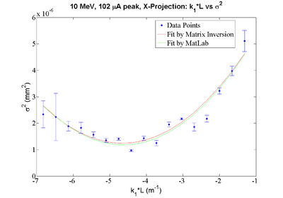
| + | [[File:HRRL_Emit_New_Fits_with_K1L_X_Projection_withErr.png | 400 px]] | ||
| + | |||
| + | |||
| + | Y Projection: | ||
| + | |||
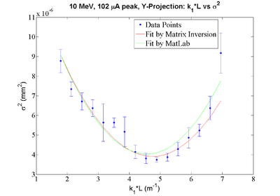
| + | [[File:HRRL_Emit_New_Fits_with_K1L_Y_Projection_withErr.png | 400 px]] | ||
| + | |||
| + | |||
| + | |||
| + | |||
| + | |||
| + | |||
| + | |||
| + | |||
| + | = Corrections for vertical calibration = | ||
| + | |||
| + | We made error when we are doing vertical calibration. When we calculate vertical calibration, we need to multiply the diameter of the circle by <math> cos45^{o} </math>. | ||
| + | |||
| + | This is the reason that we got dramatically different results in vertical and horizontal emittances. | ||
| + | |||
| + | |||
| + | |||
| + | == Errors in Converting pixels to length for Vertical == | ||
| + | |||
| + | |||
| + | {| border="1" |cellpadding="20" cellspacing="0 | ||
| + | |- | ||
| + | | || Average Horizontal Diameter (pixels) || Average Vertical Diameter (pixels) || | ||
| + | |- | ||
| + | | || <math> 90.29 \pm 0.49 </math> || <math> 59.43 \pm 0.53 </math> || | ||
| + | |- | ||
| + | | || Horizontal mm/pixels || Vertical mm/pixels || | ||
| + | |- | ||
| + | | || <math> 0.1108 \pm 0.0006 </math> || <math> 0.1683 \pm 0.0015 </math> || | ||
| + | |- | ||
| + | | || || <math> V_{cal} </math> need to be multiplied by <math> cos45^{o} </math> || | ||
| + | |- | ||
| + | | || || <math> 0.1190\pm 0.0011 </math> || | ||
| + | |- | ||
| + | |} | ||
| + | |||
| + | == New Fits with K1L == | ||
| + | |||
| + | === Considering fringe field effect with "Cheap and Dirty" way=== | ||
| + | |||
| + | ==== X Projection ==== | ||
| + | |||
| + | [[File:HRRL_Emitt_2010_Jul_Refit_After_Correcting_Calibration_Projection_X.png | 300 px]] | ||
| + | |||
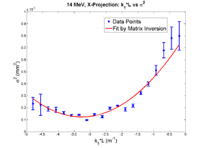
| + | x-projection: | ||
| + | |||
| + | emit=2.2 +- 1.3 mm*mrad, emit_norm=42.4 +- 25.4 mm*mrad | ||
| + | |||
| + | beta=0.72 +- 0.31, alpha=-1.23 +-0.56 | ||
| + | |||
| + | //K1*L(1/m) er K1*L sgima^2(mm) er sigma^2 | ||
| + | |||
| + | [[Media:2010_Jul_Emit_refit_data_x.txt]] | ||
| + | |||
| + | |||
| + | parabola fit for x-projection (y in mm unit): | ||
| + | |||
| + | y = (8.05126 +-0.24983) + (4.18341+-0.18968)*x + (0.64143+-0.03472)*x.*x | ||
| + | |||
| + | Data created from parabola fit | ||
| + | |||
| + | [[Media:2010_Jul_Emit_data_from_fit_x.txt]] | ||
| + | |||
| + | ==== Y Projection ==== | ||
| + | |||
| + | |||
| + | |||
| + | [[File:HRRL_Emitt_2010_Jul_Refit_After_Correcting_Calibration_Projection_Y.png | 300 px]] | ||
| + | |||
| + | |||
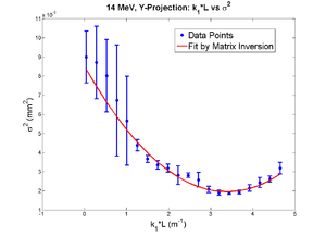
| + | y-projection: | ||
| + | |||
| + | emit=2.6 +- 2.0 mm*mrad, emit_norm=50.5 +- 38.3 mm*mrad | ||
| + | |||
| + | beta=0.54 +- 0.22, alpha=2.68 +-1.13 | ||
| + | |||
| + | |||
| + | //K1*L(1/m) er K1*L sgima^2(mm) er sigma^2 | ||
| + | |||
| + | [[Media:2010_Jul_Emit_refit_data_y.txt]] | ||
| + | |||
| + | |||
| + | parabola fit for y-projection (y in mm unit): | ||
| + | |||
| + | y = (8.51813 +-0.40098) + (-3.88142+-0.28132)*x + (0.57350+-0.04792)*x.*x | ||
| + | |||
| + | Data created from parabola fit | ||
| + | |||
| + | [[Media:2010_Jul_Emit_data_from_par_fit_y.txt]] | ||
Go back [[Positrons]] | Go back [[Positrons]] | ||
Latest revision as of 07:01, 22 October 2012
Design
New deisign: We changed to use just one magnet.
File:Emittance Test Optim File.txt
HRRL had steer magnets on itself. We don't need external steer magnets. But Dr. Chouffani said that we might need them after quads, if the quads are not on axis. He will think about it.
Beam Line design on 27th, Jul. 2010:
Optim File on 27th, Jul. 2010:
File:Emittance Test Optim File 27th Jul 2010.txt
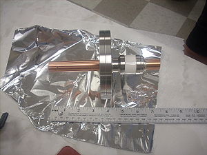
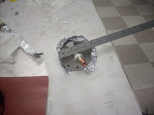
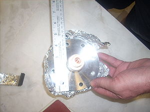
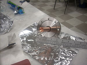
YAG (Yttrium Aluminum Garnet) Christal
Faraday Cup
Old Beam Line
Beam Line Parts
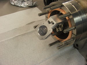
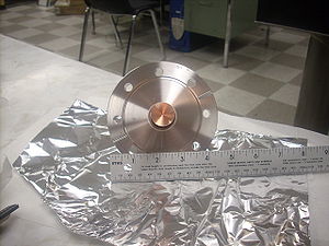
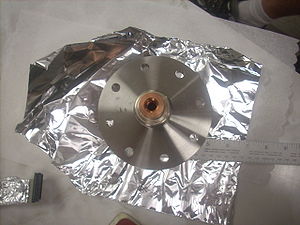
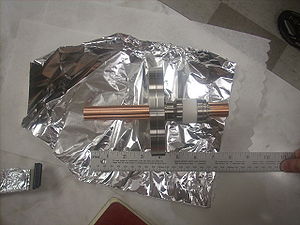
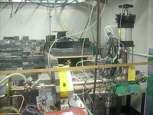
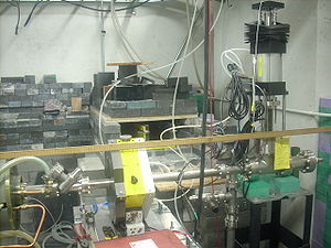
Length of the pole face of Quad2Tin z direction is 8 cm.
Constructed Beam Line for Emittance Test
Vacuum pressure on the beam line is less than torr (on 2010-July-7th).
Leveling Survey
Downstream of the beam up by 2.6 mm.
How to do Leveling Survey and Alignment with Theodolite on e- Beam Line
A. Leveling Beam Pipe
1. Put the theodolite as high as the center of the beam line at upstream. Turn theodolite up and down. If the up angle is equal to down angle from the center of the pipe, theodolite is exactly as high as beam pipe. If not, adjust theodolite, until up and down angles are equal.
2. Once first step finished, then rotate theodolite horizontally to down stream. Turn it up and down, if up and down angles are not equal, adjust the stand till they are equal.
B. How to Make Sure the Quad is Perpendicular to the Beam Line
If the distances between quads and end of cavity at any given points are equal, then quad and end of cavity are parallel. Pipe is perpendicular to the end of the cavity, thus, magnet would also be perpendicular to the pipe.
I will find at lest three random points quads and three corresponding points at the end of the cavity, make sure they are equal, then I can say, magnet is perpendicular to the beam line.
I am planning to stick a metal ruler two, so two faces are parallel.
C. Centering the Quad Magnet with Theodolite
Vertical Centering
1. Finish the step 1 in A.
2. Then turn up the theodolite from the upper edge of the pipe to the magnet hole, call this angle upper angle. Do the same at lower part, call it lower angle. If the this two angles are not equal adjust the stand till they are equal.
Horizantal Centering
We know the diameter of the pipe . So, we can calculate from the pipe to the edge of the quad as:
We need to make sure this distance is same when measure it horizontally, so that our quad is centered on the pipe. I am going to use a ruler to ...(thinking)
July 2010 Run
- Initial Accelerator Settings
E = 10 MeV Control Voltage= 4.09 V
Pulse Width <= 50 ns
Average Beam Current = least amount needed to light up YaG crystal, start at 1 mA and Rep rate of 100 Hz.
At the same time we want to do radiation test on HRRL. This is for predicting the radiation after shifting cavity to new position. Radiation test run plan is at: [1]
7/26/10
Alignment check
1.) Survey the Quad to be sure it is centered on the beam pipe
2.) survey the flag to determine if target is centered on the beam pipe
Transmission tuning
1.) Using the quads and accelerator coils, focus the beam on the YaG crystal to as fine a spot as possible. Monitor the FC during the focusing.
changed control Voltage from
Control Voltage= 4.9 V E = 16 MeV
to
4.09 V E = 10 MeV
Tune the 4 accelerator coils for max transmission.
We want to maximize the current reach the Farady Cup. This can be determined by the ratio on Channels of FC and Gun Current.
Gun current is the current on the pick up coil, which is input current for cavity. Current on Farady cup is the current reach the end of the beam line (FC is at the end of the beam line). We want to maximize the the ratio of Farady cup current to Gun current (FCC/GC), so there are more electrons will make it to the target. Thus, we enlarge our positron yield.
Basic principle: Fix three coils, change one till it maximized.
The HRRL went down after 2 hours of operation.
7/27/10
No HRRL beam time today. Chad tested the Thermatron module and believes it is not the problem. Chad will continue debugging tomorrow.
Filament
BMP format:
Wiki won't allow me to upload with bmp extension. So, I used png extension to upload. After download files, you will find they are still with bmp extension.
7/28/10
The HRRL came back around 3pm today. A capacitor in the bank was found to be the problem.
Maximize Transmission
Maximized setup according to the accelerator operator.
Beam Energy: 16 MeV
Rep Rate: 95 Hz
Pulse Width: 100 ns
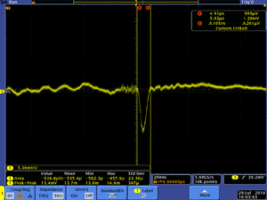
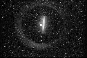
| Coil 1 upstream left/right (A) | Coil 2 upstream UP/down (A) | Coil 3 downstream up/down (A) | Coil 4 downstream left right (A) | Scope Picture | Gun Current | FC current | Ratio | Spot Size | |
| 0.1 | 0.5 | 3.1 | 0.7 |  |
Reversed the polarities on coil # 3 and coil # 4. Rep rate: 3Hz
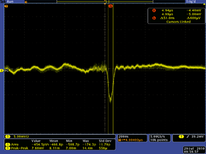
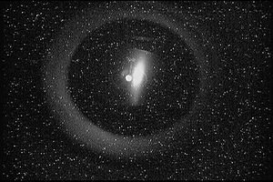
| Coil 1 upstream left/right (A) | Coil 2 upstream UP/down (A) | Coil 3 downstream up/down (A) | Coil 4 downstream left right (A) | Scope Picture | Gun Current | FC current | Ratio | Spot Size | |
| 1.2 | 1.2 | 0.0 | 3 |  |
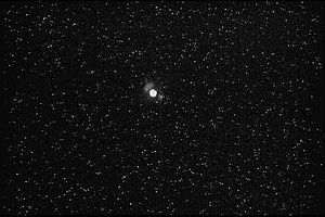
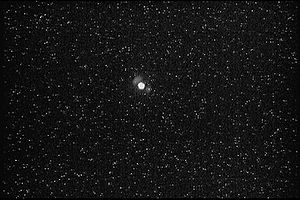
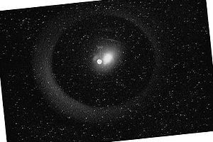
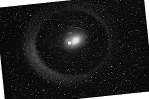
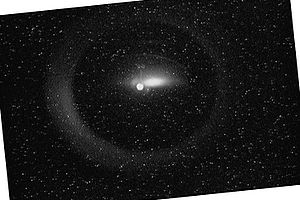
After image manipulation in GIMP to remove spot from the filament, Arne obtained reasonable projections for horizontal and vertical beam sizes ( < 2 mm). The quad was off, low rep rate to avoid saturation, 10MeV. This was the spot for the initial setup on Wednesday.
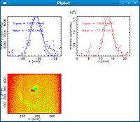
Electron beam deflection due to Earth's B-field.
It appears the the image from electrons hitting the YaG crystal is offset (to the right) compare to the image from the filament which appears near the center of the cross hairs.
Is the earths Magnetic field causing the electrons to move this far beam right?
= 0.00005 Tesla ( ) = 0.5 Gauss
E_{electron} = 10 MeV = Pc P = 10 MeV/c
Estimation using Classical Lorentz Force (forget about angle of B and V)
assuming and are orthogonal then we get the cyclotron radius
Now some Geometry.
Assuming the orbit is a circle with a 700 m radius, then the question becomes how far does the electron move to maintain the orbit if it travels 1 m in a straight line.
let
= radius of circle
= distance along the beam line
= deflection due to gravity
- Note
- is a tangent to the orbit
one can construct a right angle triangle with side of length d, the as the base and as the hypotenuse.
Then Pythagorean's theorem gives
Giving
using quadratic formula you get
since l/r is very small (1/700) we can approximate this as
for 10 MeV and a 1 m long beam pipe
where is in units of m
Radiation Footprint Measurements
Spent the remaining beam time doing radiation footprint measurements.
7/29/10
Today we first tune up the beam for max transmission.
If the above calculation is correct we can expect the electron beam to move at least 2 mm away from the center of the FC. We could test it the Earth's B-field is the cause of the deflection by watch the deflection as a function of the beam energy. If we had enough -metal we could wrap the beam pipe in it and see if the deflection goes away.
Quad Scan
First Scan
- Beam current
Second Scan (Polarity Changed)
PS Output Current to Shunt Resistance Current Conversion
PS negative connected to Quad positive.
Shunt resistance: 50 AMP, 50 MV. (PR 0050, QECO)
| PS Reading (Amps) | Shunt Resistance Voltage (mV) | Shunt Resistance Current (Amps) (Calculated) |
| 0 | 0 | 0 |
| 1 | 1 | 1 |
| 2 | 2.1 | 2.1 |
| 3 | 3.2 | 3.2 |
| 4 | 4.3 | 4.3 |
| 5 | 5.4 | 5.4 |
| 6 | 6.4 | 6.4 |
| 7 | 7.4 | 7.4 |
| 8 | 8.5 | 8.5 |
| 9 | 9.6 | 9.6 |
| 10 | 10.7 | 10.7 |
| 11 | 11.7 | 11.7 |
| 12 | 12.8 | 12.8 |
| 13 | 13.9 | 13.9 |
| 14 | 14.9 | 14.9 |
| 15 | 16 | 16 |
| 16 | 17 | 17 |
| 17 | 18.1 | 18.1 |
| 18 | 19.2 | 19.2 |
| 19 | 20.3 | 20.3 |
| 20 | 21.3 | 21.3 |
| 21 | 22.4 | 22.4 |
| 22 | 23.5 | 23.5 |
Radiation Footprint Measurements
spent noon to 3pm on radiation measurements below
HRRL_radiation_tests#29_Jul_2010
Earth's B-field effect
It the above calculation on the effects of the Earth's Magnetic field on a the electron beam is correct then we should see the amount of deflection depend inversely on the electron's momentum (1/P).
So lets take a few pictures at the energy exterma to see how far the electron spot moves away from the filament image on the crystal.
| E beam (V gun) | YaG picture | Beam Spot posiiton (arb offset) | |
| 5 | 100 px | ||
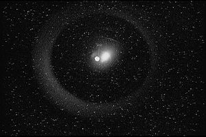
| 10 (4.09 V) |  |
-31.8 .1 mm | |
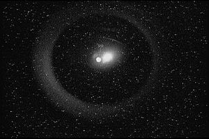
| 16 (4.9 V) |  |
-32.0 0.1 mm |
We did not see the beam spot move when the energy was changed from 10 MeV to 16 MeV, but going to lower energy definitely moved the beam spot farther away from the center filament image that is located on the YaG crystal cross hairs.
Maximize Transmission
Change the linac coils to determine a setting which delivers the maximum current to the FC and has a reasonable spot size on the YaG viewer.
| Coil 1 upstream left/right (A) | Coil 2 upstream UP/down (A) | Coil 3 downstream up/down | Coil 4 downstream left right | Scope Picture | Gun Current | FC current | Ratio | YaG Image |
| 0 | 0.6 | 1.8 | 2.7 |
| Coil 1 upstream left/right (A) | Coil 2 upstream UP/down (A) | Coil 3 downstream up/down | Coil 4 downstream left right | Scope Picture | Gun Current | FC current | Ratio | YaG Image |
| 0 | 0.6 | 1.8 | 2.7 | 100px | 100px |
a.) Does a small beam spot size on the crystal give maximum FC signal?
b.) Is there a point where the spot size changes and you can't resolve a change in the FC output?
c.) Remove the YaG target and determine if above observations are unchanged.
Pickup Coil Calibration
2.) After tuning the beam to deliver the Maximum beam current to the FC, measure the FC and green pickup coil output as a function of current by integrating the pulse with an oscilloscope.
| FC output | Green Pickup Coil output | Spot on Crystal | Scope |
| (mA) | (mA) | ||
| 0.5 |  |

| |
| 1 |  |

| |
| 1.5 |  |

| |
| 2 |  |

| |
| 2.5 |  |

| |
| 3 |  |

| |
| 3.5 |  |

| |
| 4 |  |

| |
| 4.5 |  |

| |
| 5 |  |

| |
| 5.5 |  |

| |
| 6 |  |

|
a.) does the FC output change with rep rate? It should not but maybe there is loss at high rates?
Quad scan
Tune the beam so a change in the quad B-field does not cause a deflection.
First attempt to measure the spot size change as a function of Quad current
| Quad Current | Beam Spot RMS (0 degrees= Left/right) | Beam Spot RMS (90 degrees= Up/Down) |
| (Amps) | (mm) | (mm) |
Shall we do both polarities?
Imaging
Background subtraction
The filament produces at least a 2 mm diameter spot on the YaG crystal. Beam dominates the image.
7/30/10
At 4pm yesterday we attempted to measure the emittance at high currents of 10 mA, previous measurements were at 0.3 mA. The beam spot became larger than the 1" YaG target holder. This would make emittance measurements impossible.
In order to measure the emittance above 1 mA we will need to insert a doublet as close to the accelerator entrance as possible. Since this would not be done by today we decided to cancel today's beam time and work on the next emittance measurement.
The YaG camera saturated at about 0.6 mA of beam current (our measurements were made at about 0.3 mA). Perhaps we should use a thin Aluminum target instead of the YaG crystal for high current measurements.
We were able to Trigger the GigE camera. We should use this next time.
Imaging scratch area
After image manipulation in GIMP to remove spot from filament. Obtained reasonable projections for horizontal and vertical beam sizes. The quad was off, low rep rate to avoid saturation, 10MeV. This was the spot for the initial setup on Wednesday.
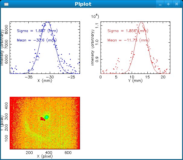
Data Analysis
Root Code: File:Pixle.C
The cut is changed from circular to elliptical on Sep. 23rd, 2010.
Rotating the Image
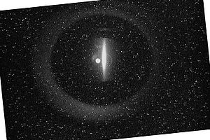
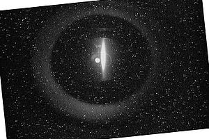
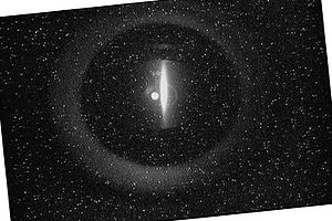
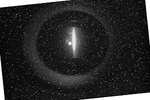
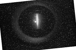
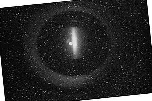
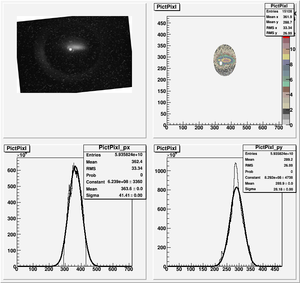
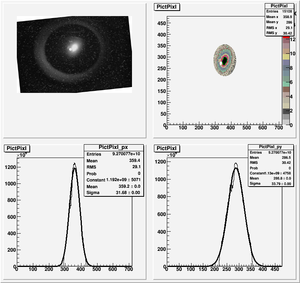
Images need to be rotated -6 degree, so cross at center of the crystal is perpendicular to the image. Here are the rotated images
1st Scan
2nd Scan
Polarity was switched from 1st scan.
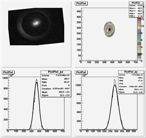
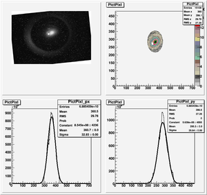
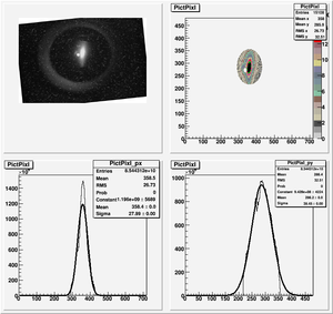
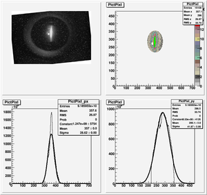
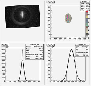
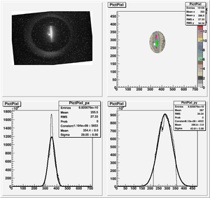
Fits for Beam Spot Projection
1st Scan
2nd Scan
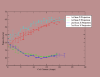
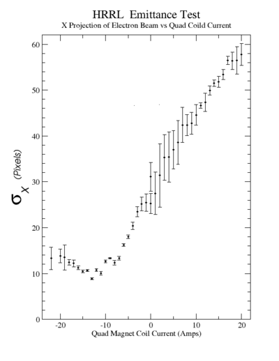
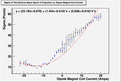
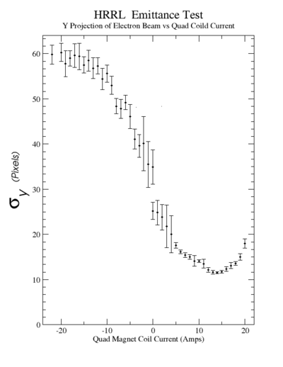
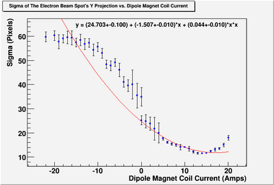
Coil Current vs Beam Spot Projection Gaussian Fit's Sigma
1st Scan
| Coil Current Reading on PS (Amps) | Coil Current Reading From Shunt Resistance (Amps) | X Projection Sigma (pixels) | Y Projection Sigma (pixels) |
| 0 | 0 | 30.28 | 30.69 |
| 1 | 1 | 31.6 | 29.81 |
| 1.4 | 32.3 | 29.37 | |
| 2 | 2.1 | 32.93 | 2864 |
| 3 | 3.2 | 34.45 | 27.85 |
| 4 | 4.3 | 35.51 | 27.3 |
| 5 | 5.4 | 36.28 | 27.06 |
| 6 | 6.4 | 37.22 | 26.52 |
| 7 | 7.4 | 38.14 | 26.8 |
| 8 | 8.5 | 38.89 | 26.97 |
| 9 | 9.6 | 38.59 | 28.29 |
| 10 | 10.7 | 39.97 | 27.44 |
| 11 | 11.7 | 39.8 | 27.72 |
| 12 | 12.8 | 40.35 | 27.67 |
| 13 | 13.9 | 40.06 | 27.67 |
| 14 | 14.9 | 40.2 | 27.76 |
| 15 | 16 | 40.26 | 27.96 |
| 16 | 17 | 40.84 | 27.81 |
| 17 | 18.1 | 41.41 | 27.93 |
| 18 | 19.2 | 41.55 | 28.12 |
| 19 | 20.3 | 41.41 | 28.18 |
| 20 | 21.3 | 42.25 | 28.58 |
2nd Scan
| Coil Current Reading on PS (Amps) | Coil Current Reading From Shunt Resistance (Amps) | X Projection Sigma (pixels) | Y Projection Sigma (pixels) |
| 0 | 0 | 31.68 | 33.79 |
| 1 | 1 | 30.51 | 34.77 |
| 2 | 2.1 | 29.72 | 36.33 |
| 3 | 3.2 | 28.81 | 37.6 |
| 4 | 4.3 | 28.11 | 38.3 |
| 5 | 5.4 | 27.99 | 38.45 |
| 6 | 6.4 | 27.78 | 39.73 |
| 7 | 7.4 | 28.07 | 39.32 |
| 8 | 8.5 | 27.91 | 39.31 |
| 9 | 9.6 | 28.38 | 41.08 |
| 10 | 10.7 | 28.62 | 41.87 |
| 11 | 11.7 | 28.66 | 41.52 |
| 12 | 12.8 | 28.91 | 42.31 |
| 13 | 13.9 | 28.8 | 42.16 |
| 14 | 14.9 | 28.95 | 42.41 |
| 15 | 16 | 29.06 | 42.58 |
| 16 | 17 | 29.27 | 42.95 |
| 17 | 18.1 | 29.15 | 43.26 |
| 18 | 19.2 | 29.01 | 42.98 |
| 19 | 20.3 | 29.05 | 42.61 |
| 20 | 21.3 | 28.93 | 43.63 |
| 22 | 23.5 | 29.08 | 44.39 |
Multi-Fits for Beam Spot Projection
Multi-Fits 1st Scan
Naming the photos: Rotated_HRRL_Emit_Test_Quad_Scan_First_20Amp_Multi_Fit7 -> RHETQSF20AMF7
| Coild Current (Amps) | 1st Fit | 2nd Fit | 3rd Fit | 4th Fit | 5th Fit | 6th Fit | 7th Fit | Mean and Error |
| 0 | ||||||||
| 1 | ||||||||
| 2 | ||||||||
| 3 | ||||||||
| 4 | ||||||||
| 5 | ||||||||
| 6 | ||||||||
| 7 | ||||||||
| 8 | ||||||||
| 9 | ||||||||
| 10 | ||||||||
| 11 | ||||||||
| 12 | ||||||||
| 13 | ||||||||
| 14 | ||||||||
| 15 | ||||||||
| 16 | ||||||||
| 17 | ||||||||
| 18 | ||||||||
| 19 | ||||||||
| 20 |
Multi-Fits 2nd Scan
Naming the photos: Rotated_HRRL_Emit_Test_Quad_Scan_Second_22Amp_Multi_Fit7 -> RHETQSS22AMF7
| Coild Current (Amps) | 1st Fit | 2nd Fit | 3rd Fit | 4th Fit | 5th Fit | 6th Fit | 7th Fit | Mean and Error |
| 0 | ||||||||
| 1 | ||||||||
| 2 | ||||||||
| 3 | ||||||||
| 4 | ||||||||
| 5 | ||||||||
| 6 | ||||||||
| 7 | ||||||||
| 8 | ||||||||
| 9 | ||||||||
| 10 | ||||||||
| 11 | ||||||||
| 12 | ||||||||
| 13 | ||||||||
| 14 | File:RHETQSS14AMF3.png | |||||||
| 15 | ||||||||
| 16 | ||||||||
| 17 | ||||||||
| 18 |  |
|||||||
| 19 | ||||||||
| 20 | ||||||||
| 22 |
Current -vs- Sigma Data Files
First Scan:
File:HRRL Emitt Current vs Sigma 1stScan x.txt
File:HRRL Emitt Current vs Sigma 1stScan y.txt
Second Scan:
File:HRRL Emitt Current vs Sigma 2ndScan x.txt
File:HRRL Emitt Current vs Sigma 2ndScan y.txt
Current vs Sigma:
X projections:
File:HRRL Emitt Current vs Sigma Projections x.txt
Fit:
P-value of this fit is less than 0.000001.
Y projections:
File:HRRL Emitt Current vs Sigma Projections y.txt
Fit:
P-value of this fit is less than 0.000001.
Next step:
calibrate: mm/pxiel
Parabola: All the x projections makeup one parabola, and y projections makeup one parabola. Put them in together.
Converting pixels to length
Diameter of circle inside crystal is 10 mm.
Convert the pictures to a histogram and measure pixels that way
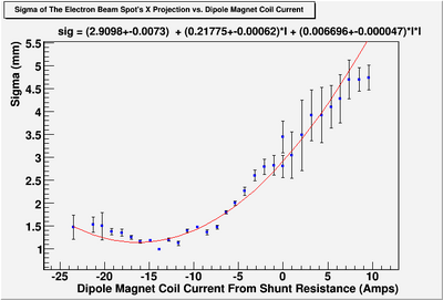
Sigma (in mm) vs Dipole Coil Current (on Shunt Resistance)
X Projection
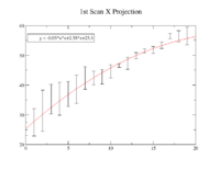
The fit is:
p-value is less than 0.000001
For a parabola , the corresponding to the minimum is:
.
So,
and
.
.
.
So,
Y Projection
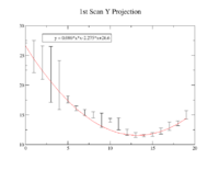
The fit is:
p-value is less than 0.000001
.
So,
.
.
So,
Conclusions
For X projection: , and
For X projection: , and
Emittance
Quadrupole Strength:
g here is the gradient of the qudrupole. p is the momentum of the e- beam.
In our case, energy of the beam is 0.01 GeV and gap between dipole center and pole face is 1 inch.
So,
According to File:Emit Meas DAFNE Linac e Beam.pdf, for the case of quadruple scanning one quadrupole and screen, the emittance related to the quadrupole strength.
Transfer Matrix for 1uaruople \tilde{Q} and screen (drift space?) \tilde{S} consist the transfer matrix of the whole system as:
is the distance between quadrupole and screen.
If I have a fit:
Then,
Two fits are:
Dr. Kim's Suggestion in his email
from	Yujong Kim <yjkim@isu.edu>
to	Sadiq Setiniyaz <sadik82@gmail.com>
cc	Dr Forest <tforest@athena.physics.isu.edu>
date	Fri, Oct 8, 2010 at 6:44 AM
subject	Re: Quad Scan Parameters
Dear Sadiq,

Many thanks,

I re-checked your QM scan fitting plot (final plots on emittance mewasurement).

Your fitting range too wide (-20 < k < 50).

Please fit again with a narrower range (+10 < k < 50).
Then, you can get much beautiful results.
Normally, we fit for only one k sign (positive or negative).
Yujong Kim
Here are results after doing Dr. Kim's suggested fit.
Note: I also corrected the distance S12 to the distance between quad center and screen (I originally did from the end of the quad to the screen, this is wrong).
For X projection
Minimum ChiSqrd is: 129.749
The fit is:
sig^2 = (7.82463e-06+-2e-08) + (4.23945e-07+-1e-09)*k + (6.82167e-09+-1e-10)*k*k
Probability of obtaining data at least as incompatible with distribution as the data actually observed is 0.000000 A = 7.82463e-06, B = -0.0270904, C = 1.07925e-09, S12=0.64. Geometrical Emittance: 2.24354e-07 (m*rad), Normalized Emittance: 4.39048e-06 (m*rad).
Data file contains: Number-of-points B-Field-Strength Error-on-B-Field-Strength Sigma^2 Error-on-Sigma^2
File:HRRL Emit Parbola Fit Xaxis as BfieldStrength.txt
For Y projection
Minimum ChiSqrd is: 25.3174
The fit is:
sig^2 = (1.71755e-05+-8e-08) + (-8.38108e-07+-3e-09)*k + (1.3229e-08+-1e-10)*k*k
Probability of obtaining data at least as incompatible with distribution as the data actually observed is 0.000000 A = 1.71755e-05, B = 0.0243983, C = 3.00479e-09, S12=0.64. Geometrical Emittance: 5.54629e-07 (m*rad), Normalized Emittance: 1.08538e-05 (m*rad).
Data file contains: Number-of-points B-Field-Strength Error-on-B-Field-Strength Sigma Error-on-Sigma
File:HRRL Emit Parbola Fit Yaxis as BfieldStrength.txt
Data ROOTSYS Fit Script
File:ROOTSCRIPT for HRRL Emittace.C
Emittance Results for HRRL at 10 MeV and 102 micro Amp peak
File:Emmitance HRRL 1mA 10-14-10.xmgrace.txt
Automatic Script to plot RMS
ROOT
How does the fit look when using the script below.
Working on it.
You should do background subtraction instead of cutting out the spot.

 2 bugs remain till Spe 24th. 1. entries; 2. Sub->Draw();
Running Parabola_Fit_for_AutoRMS.C will run AutoRMS.C and do the fits.
File:Parabola Fit for AutoRMS.C
This 2 programs and pictures for data can be downloaded at: [2]
MATLAB
These MATLAB scripts will do Gaussian fits for beam spots and get rms beam size on x and projections (by Gauss_Fit.m). These rms values will be passed on (to Emit_Parabola_Fit_kl_YProjection.m and Emit_Parabola_Fit_kl_YProjection.m) to fit parabola. Parabola fit will be plotted,and emittances, normalized emittances, beta functions, alpha functions will given at the end.
File:Emit Parabola Fit kl XProjection.txt
File:Emit Parabola Fit kl YProjection.txt
Alternative Analysis from the East Cost
Emittance/TWISS parameter extraction
New Fits with K1L
No Fringe Field Effect
We want to do new fits with K1L. K1 is quadrupole strength and L is the thickness of the quadrupole. We will do it for the data we got previously. They are the following two data sets.
At this step, we will ignore fringe field effect, we want to consider it later.
need uncertainties in plots below
The uncertainties are difficult to believe because they are so small (< 0.1% !)
Redo you plots so they look like the ones below in terms of line boldness and quality. Identify the fit parameters and their error as well as a measurement of the goodness of fit.
https://wiki.iac.isu.edu/index.php/File:Emittance_HRRL_1mA.png
Data files contains:
Number-of-points B-Field-Strength Error-on-B-Field-Strength Sigma^2 Error-on-Sigma^2
File:HRRL Emit Parbola Fit Xaxis as BfieldStrength.txt
File:HRRL Emit Parbola Fit Yaxis as BfieldStrength.txt
X-Projection:
Fit Parameters by MATLAB:
y = 0.00000784 + (0.00000288)*x + 0.00000031*x*x
Fit Parameters by Matrix Inversion:
y = (0.00000781+-0.00000027) + (0.00000282+-0.00000014)*x + (0.00000030+-0.00000002)*x*x
P-value = 7.6238e-21
Y-Projection:
Fit Parameters by MATLAB:
y = 0.00001766 + (-0.00000599)*x + 0.00000066*x*x
Fit Parameters by Matrix Inversion:
y = (0.00001717+-0.00000084) + (-0.00000558+-0.00000041)*x + (0.00000059+-0.00000005)*x*x
P-value =  0.020964
geometrical emittance: normalized emittance:
X Projection:
Y Projection:
Corrections for vertical calibration
We made error when we are doing vertical calibration. When we calculate vertical calibration, we need to multiply the diameter of the circle by .
This is the reason that we got dramatically different results in vertical and horizontal emittances.
Errors in Converting pixels to length for Vertical
| Average Horizontal Diameter (pixels) | Average Vertical Diameter (pixels) | ||
| Horizontal mm/pixels | Vertical mm/pixels | ||
| need to be multiplied by | |||
New Fits with K1L
Considering fringe field effect with "Cheap and Dirty" way
X Projection
x-projection:
emit=2.2 +- 1.3 mm*mrad, emit_norm=42.4 +- 25.4 mm*mrad
beta=0.72 +- 0.31, alpha=-1.23 +-0.56
//K1*L(1/m) er K1*L sgima^2(mm) er sigma^2
Media:2010_Jul_Emit_refit_data_x.txt
parabola fit for x-projection (y in mm unit):
y = (8.05126 +-0.24983) + (4.18341+-0.18968)*x + (0.64143+-0.03472)*x.*x
Data created from parabola fit
Media:2010_Jul_Emit_data_from_fit_x.txt
Y Projection
y-projection:
emit=2.6 +- 2.0 mm*mrad, emit_norm=50.5 +- 38.3 mm*mrad
beta=0.54 +- 0.22, alpha=2.68 +-1.13
//K1*L(1/m) er K1*L sgima^2(mm) er sigma^2
Media:2010_Jul_Emit_refit_data_y.txt
parabola fit for y-projection (y in mm unit):
y = (8.51813 +-0.40098) + (-3.88142+-0.28132)*x + (0.57350+-0.04792)*x.*x
Data created from parabola fit
Media:2010_Jul_Emit_data_from_par_fit_y.txt
Go back Positrons
