Difference between revisions of "DV MollerTrackRecon"
| (51 intermediate revisions by the same user not shown) | |||
| Line 1: | Line 1: | ||
| − | = | + | =Phi shifts= |
| + | ==gcard== | ||
| − | |||
| − | |||
<pre> | <pre> | ||
| − | + | <gcard> | |
| − | |||
| − | |||
| − | < | ||
| + | <detector name="../../../../../clas12/fc/forwardCarriage" factory="TEXT$ | ||
| + | <detector name="../../../../../clas12/dc/dc" factory="TEXT" $ | ||
| + | <detector name="../../../../../clas12/ec/ec" factory="TEXT" $ | ||
| + | <detector name="../../../../../clas12/ctof/ctof" factory="TE$ | ||
| + | <detector name="../../../../../clas12/ftof/ftof" factory="TE$ | ||
| + | <detector name="../../../../../clas12/htcc/htcc" factory="TE$ | ||
| + | <detector name="../../../../../clas12/pcal/pcal" factory="TE$ | ||
| + | <option name="BEAM_P" value="e-, 6.0*GeV, 30.0*deg, 10*deg"/> | ||
| + | <option name="SPREAD_P" value="5.5*GeV, 25*deg, 180*deg"/> | ||
| + | <option name="SCALE_FIELD" value="clas12-torus-big, -1.0"/> | ||
| + | <option name="HALL_FIELD" value="clas12-solenoid"/> | ||
| + | <option name="SCALE_FIELD" value="clas12-solenoid, 1.0"/> | ||
| + | <option name="OUTPUT" value="evio,eg12.ev"/> | ||
| − | + | </gcard> | |
| − | |||
| − | |||
| − | |||
| − | |||
| − | |||
| − | |||
| − | |||
| − | |||
| − | |||
| − | |||
| − | |||
| − | |||
| − | |||
| − | |||
| − | |||
| − | |||
| − | |||
| − | |||
| − | |||
| − | |||
| − | |||
| − | |||
| − | |||
| − | |||
| − | |||
| − | |||
| − | |||
| − | |||
| − | |||
| − | |||
| − | |||
| − | |||
| − | |||
| − | |||
| − | |||
| − | |||
| − | |||
| − | |||
| − | |||
| − | |||
| − | |||
| − | |||
| − | |||
| − | |||
| − | |||
| − | |||
| − | |||
| − | |||
| − | |||
| − | |||
| − | |||
| − | |||
| − | |||
| − | |||
| − | |||
| − | |||
| − | |||
| − | |||
| − | |||
| − | |||
| − | |||
| − | |||
| − | |||
| − | |||
| − | |||
| − | |||
| − | |||
| − | |||
| − | |||
| − | |||
| − | |||
| − | |||
| − | |||
| − | |||
| − | |||
| − | |||
| − | |||
| − | |||
| − | |||
| − | |||
| − | |||
| − | |||
| − | |||
| − | |||
| − | |||
| − | |||
| − | |||
| − | |||
| − | |||
| − | |||
| − | |||
| − | |||
| − | |||
| − | |||
| − | |||
| − | |||
| − | |||
| − | |||
| − | |||
| − | |||
| − | |||
| − | |||
| − | |||
| − | |||
| − | |||
| − | |||
| − | |||
| − | |||
| − | |||
| − | |||
| − | |||
| − | |||
| − | |||
| − | |||
| − | gcard | ||
| − | |||
| − | |||
| − | |||
| − | |||
| − | |||
| − | |||
| − | |||
| − | |||
| − | + | </pre> | |
| − | |||
| − | |||
| − | |||
| − | |||
| − | |||
| − | |||
| − | |||
=Cross-section = | =Cross-section = | ||
| Line 155: | Line 34: | ||
===Prepare Data=== | ===Prepare Data=== | ||
| − | Using the existing Moller scattering data from a GEANT simulation of | + | Using the existing Moller scattering data from a GEANT simulation of 4E8 incident electrons, a file of just scattered momentum components can be constructed using: |
<pre> | <pre> | ||
| Line 176: | Line 55: | ||
===Run for Necessary Amount to match Cross Section=== | ===Run for Necessary Amount to match Cross Section=== | ||
| − | <center>[[File: | + | <center>[[File:Combo3.png]]</center> |
Using the above plot for the target material, we can find the relative amount that each Theta angle should observe for this process which gives a [[known Moller differential cross section]]. | Using the above plot for the target material, we can find the relative amount that each Theta angle should observe for this process which gives a [[known Moller differential cross section]]. | ||
| Line 248: | Line 127: | ||
we should find the change in phi needed to give an evenly distributed distribution around the xy plane for a given Theta angle. | we should find the change in phi needed to give an evenly distributed distribution around the xy plane for a given Theta angle. | ||
| + | |||
| + | <center>[[File:UniformPhi.png]]</center> | ||
===Alter Phi Angles=== | ===Alter Phi Angles=== | ||
| − | + | From a C++ program, random Energies and Angle Theta are read from the 2-D histogram created above. Using Relativistic kinematics for CM frame, a 4-momenta vector for the Moller electron is created. Using the properties of the CM frame, a 4-momenta vector for the scattered electron is created. Using the relative counts for number of events at a given angle theta in the CM frame, multiple copies of the Moller CM 4-momenta vector are created. Since the rotation of the angle Phi does not alter the z or total momentum, the same paired version of the scattered electron 4-momenta vector are transfered over from the Moller. | |
| − | + | [[Altering Phi Angles]] | |
| − | |||
| − | |||
| − | |||
| − | |||
| − | |||
| − | |||
| − | |||
| − | |||
| − | |||
| − | |||
| − | |||
| − | |||
| − | |||
| − | |||
| − | |||
| − | |||
| − | |||
| − | |||
| − | |||
| − | |||
| − | |||
| − | |||
| − | |||
| − | |||
| − | |||
| − | |||
| − | |||
| − | |||
| − | |||
| − | |||
| − | |||
| − | |||
| − | |||
| − | |||
| − | |||
| − | |||
| − | |||
| − | |||
| − | |||
| − | |||
| − | |||
| − | |||
| − | |||
| − | |||
| − | |||
| − | |||
| − | |||
| − | |||
| − | |||
| − | |||
| − | |||
| − | |||
| − | |||
| − | |||
| − | |||
| − | |||
| − | |||
| − | |||
| − | |||
| − | |||
| − | |||
| − | |||
| − | |||
| − | |||
| − | |||
| − | |||
| − | |||
| − | |||
| − | |||
| − | |||
| − | |||
| − | |||
| − | |||
| − | |||
| − | |||
| − | |||
| − | |||
| − | |||
| − | |||
| − | |||
| − | |||
| − | |||
| − | |||
| − | |||
| − | |||
| − | |||
| − | |||
| − | |||
| − | |||
| − | |||
| − | |||
| − | |||
| − | |||
| − | |||
| − | |||
| − | |||
| − | |||
| − | |||
| − | |||
| − | |||
| − | |||
| − | |||
| − | |||
| − | |||
| − | |||
| − | |||
| − | |||
| − | |||
| − | |||
| − | |||
| − | |||
| − | |||
| − | |||
| − | |||
| − | |||
| − | |||
| − | |||
| − | |||
| − | |||
| − | |||
| − | |||
| − | |||
| − | |||
| − | Using the | + | Using two paired 4-momenta vectors in the CM frame, we can rotate them from the "CM-final" state to the "CM-initial" state by having the total momentum of each vector being held only in the z-component as would be expected for two colliding particles (<math>\theta = 0, \phi = 0</math>). From this, a Lorentz boost can be performed to find the 4-vectors in the Lab frame for an incoming electron or various energies striking a stationary electron. With the boost vector a second Lorentz boost can be performed from the Final CM Frame to the Final Lab Frame. In this state, the phi distribution is unaffected by the Lorentz boost (perpendicular to direction of relativistic motion), while the theta angle is transformed. |
| + | 10 separate trials were run for 10,000 events each. | ||
| + | The histograms of Momentum, Angle Theta and Phi for the scattered and Moller electron in both the final lab frame and final CM frame were combined using: | ||
| − | < | + | <pre>hadd -f Total_MakeCM_4e9.root set1/MakeCM_4e9.root set2/MakeCM_4e9.root set3/MakeCM_4e9.root set4/MakeCM_4e9.root set5/MakeCM_4e9.root set6/MakeCM_4e9.root set7/MakeCM_4e9.root set8/MakeCM_4e9.root set9/MakeCM_4e9.root set10/MakeCM_4e9.root</pre> |
| + | The Phi distribution for the CM and Lab frame. | ||
| − | |||
| + | [[File:MolPhiLab.png]][[File:MolPhiCM.png]] | ||
| − | |||
| + | Their LUND files were combined using | ||
| − | < | + | <pre>cat set1/Extra_Phi.LUND set2/Extra_Phi.LUND set3/Extra_Phi.LUND set4/Extra_Phi.LUND set5/Extra_Phi.LUND set6/Extra_Phi.LUND set7/Extra_Phi.LUND set8/Extra_Phi.LUND set9/Extra_Phi.LUND set10/Extra_Phi.LUND >Total_Extra_Phi.LUND</pre> |
| + | resulting in a LUND file that was 13309755 lines in length, which equates to 4436585 entries. This was divided into 177 file parts of 75000 each. The first set from the original data set is shown below. | ||
| + | <pre>split -a 4 -d -l 75000 Total_Extra_Phi.LUND Phi_Parts_</pre> | ||
| − | |||
| + | <center>[[File:File1of177.png]]</center> | ||
| + | It was shown earlier that the differential cross section scale is <math>\frac{d\sigma}{d\Omega}\approx 16.2\times 10^{-2}mb=16.2\mu b</math> | ||
| − | + | For an Ammonia target: | |
| + | :::::<math>\rho_{target}\times l_{target}=\frac{.8 g}{1 cm^3}\times \frac{1 mole}{17 g} \times \frac{6\times10^{23} atoms}{1 mole} \times \frac{1 cm}{ } \times \frac{10^{-24} cm^2}{barn} =2.82\times 10^{-2} barns</math> | ||
| + | If the beam had 4E9 incident electrons, the differential cross-section would be found with, | ||
| − | + | :::::<math>\frac{1}{\rho_{target}\times l_{target} \times 4\times 10^9}=8.87\times 10^{-9} barns=.00887 \mu b</math> | |
| + | Since extra Phi angles have been produced obviously a larger number of incident electrons would be needed. Looking at the number Moller events are created for 1E6, 1E7, and 4E9 incident electrons, we can estimate the number of incident electrons needed for the number of extra Phi angles produced. | ||
| − | {| | + | {| border=1 |
| − | |+ | + | |+ Moller Events per Incident Electrons |
|- | |- | ||
| − | ! | + | ! # of Incident Electrons |
| − | + | ! # of Moller Events | |
| − | + | ! # of E>500MeV | |
| − | |||
| − | ! | ||
| − | ! | ||
|- | |- | ||
| − | | | + | | 1e6 |
| − | | | + | | 38343 |
| − | | | + | | 134 |
| − | |||
| − | |||
| − | |||
|- | |- | ||
| − | | | + | | 1e7 |
| − | | | + | | 383633 |
| − | | | + | | 1490 |
| − | |||
| − | |||
| − | |||
|- | |- | ||
| − | | | + | | 4e9 |
| − | | | + | | 12444898 |
| − | | | + | | 48548 |
| − | |||
| − | |||
| − | |||
| − | |||
| − | |||
| − | |||
| − | |||
| − | |||
| − | |||
| − | |||
|} | |} | ||
| − | |||
| − | |||
| − | + | This shows a trait of providing around 100 Moller electrons of Energy greater that 500 MeV for about 1 million incident electrons of Energy 11 GeV. Since the boosting of the number of Phi angles leaves around 4431573 Moller electrons with Energy greater than 500 MeV, this would imply around 4e10 incident electrons of Energy 11 GeV. | |
| + | Using the same expression, but this time for 4e10 incident electrons, | ||
| + | :::::<math>\frac{1}{\rho_{target}\times l_{target} \times 4\times 10^{10}}=8.87\times 10^{-10} barns=.000887 \mu b</math> | ||
| + | Rebining the histogram to account for the unequal weighting of the bins outlined in the table above | ||
| − | < | + | <pre>TH1F *Combo=new TH1F("TheoryExperiment","Theoretical and Experimental Differential Cross-Section CM Frame",360,90,180); |
| + | Combo->Add(MolThetaCM,8.87e-10); | ||
| + | Combo->Draw(); | ||
| + | Double_t Bins[16]={90,100,110,120,130,135,140,142,144,146,148,150,152,154,156,180}; | ||
| + | hnew=Combo->Rebin(15,"hnew",Bins); | ||
| + | hnew->Draw(); | ||
| + | Theory->Draw("same");</pre> | ||
| − | + | [[File:Extended_DiffXSect_TheoryExperiment.png]] | |
| + | ===Running LUND files in GEMC=== | ||
| − | + | Since the LUND file is limited to 75000 lines, the gemc will have to be run in batch mode; | |
| + | Creating a batch directory, with two subdirectories; 1)Phi_Parts, 2)submit. | ||
| − | |||
| + | '''1)'''Once the LUND file is broken into 178 parts, they can have the LUND extension added by: | ||
| + | <pre>prename 's/(Phi_Parts_\d{4})/$1.LUND/' Phi_Parts_*</pre> | ||
| − | + | Placing each of these files into its own directory, within a directory named Phi_Parts | |
| + | <pre>find . -name "*.LUND" -exec sh -c 'mkdir "${1%.*}" ; mv "$1" "${1%.*}" ' _ {} \;</pre> | ||
| + | '''2)'''Creating the submit directory, and using a c++ program, creating the needed 178 | ||
| − | < | + | <pre>#include <iomanip> |
| + | #include <sstream> | ||
| + | #include <iostream> | ||
| + | #include <fstream> | ||
| + | using namespace std; | ||
| + | void submit() { | ||
| − | < | + | for(int a=0;a<2;a++) |
| + | { | ||
| + | for(int b=0;b<10;b++) | ||
| + | { | ||
| + | for(int c=0;c<10;c++) | ||
| + | { | ||
| + | string filename="submit0"; | ||
| + | stringstream hundreds; | ||
| + | hundreds << a; | ||
| + | stringstream tens; | ||
| + | tens << b; | ||
| + | stringstream ones; | ||
| + | ones << c; | ||
| + | string fullname=""; | ||
| + | fullname=filename + hundreds.str() + tens.str() + ones.str(); | ||
| + | // cout << fullname << "\n"; | ||
| + | |||
| + | ofstream myfile; | ||
| + | myfile.open(fullname.c_str()); | ||
| + | |||
| + | |||
| + | myfile << "#!/bin/sh\n"; | ||
| + | myfile << "#PBS -l nodes=1\n"; | ||
| + | myfile << "#PBS -A FIAC\n"; | ||
| + | myfile << "#PBS -M vanwdani@isu.edu\n"; | ||
| + | myfile << "#PBS -m abe\n"; | ||
| + | myfile << "#\n"; | ||
| + | myfile << "cd /home/lds/src/CLAS/GEMC\n"; | ||
| + | myfile << "tcsh\n"; | ||
| + | myfile << "source setup\n"; | ||
| + | myfile << "cd /home/lds/src/GEANT/geant4.9.6/geant4.9.6-install/bin/geant4.sh\n"; | ||
| + | myfile << "cd /home/vanwdani/src/GEANT4/geant4.9.6/Simulations/Research/Moller/batch/Phi_Parts/Phi_Parts_0"; | ||
| + | myfile <<a<<b<<c<<"\n"; | ||
| + | myfile << "gemc -USE_GUI=0 -Hall_Material=\"Vacuum\" -INPUT_GEN_FILE=\"LUND, Phi_Parts_0"; | ||
| + | myfile <<a<<b<<c; | ||
| + | myfile << ".LUND\" -N=75000 eg12.gcard\n"; | ||
| + | myfile << "~/src/CLAS/coatjava-1.0/bin/clas12-reconstruction -i eg12.ev -config DCHB::torus=1.0 "; | ||
| + | myfile << "-config DCHB::solenoid=0.0 -config DCTB::kalman=true -o eg12_rec.ev -s DCHB:DCTB:EC:FTOF:EB\n"; | ||
| + | myfile << "~/src/CLAS/coatjava-1.0/bin/rungroovy Analysis.groovy eg12_rec.0.evio\n"; | ||
| + | |||
| + | |||
| + | myfile.close(); | ||
| + | } | ||
| + | } | ||
| + | } | ||
| + | |||
| + | }</pre> | ||
| + | |||
| + | This creates the submitXXXX file | ||
| + | |||
| + | <pre>#!/bin/sh | ||
| + | #PBS -l nodes=1 | ||
| + | #PBS -A FIAC | ||
| + | #PBS -M vanwdani@isu.edu | ||
| + | #PBS -m abe | ||
| + | # | ||
| + | cd /home/lds/src/CLAS/GEMC | ||
| + | tcsh | ||
| + | source setup | ||
| + | cd /home/lds/src/GEANT/geant4.9.6/geant4.9.6-install/bin/geant4.sh | ||
| + | cd /home/vanwdani/src/GEANT4/geant4.9.6/Simulations/Research/Moller/batch/Phi_Parts/Phi_Parts_0000 | ||
| + | gemc -USE_GUI=0 -Hall_Material="Vacuum" -INPUT_GEN_FILE="LUND, Phi_Parts_0000.LUND" -N=75000 eg12.gcard | ||
| + | ~/src/CLAS/coatjava-1.0/bin/clas12-reconstruction -i eg12.ev -config DCHB::torus=1.0 -config DCHB::solenoid=0.0 -config DCTB::kalman=true -o eg12_rec.ev -s DCHB:DCTB:EC:FTOF:EB | ||
| + | ~/src/CLAS/coatjava-1.0/bin/rungroovy Analysis.groovy eg12_rec.0.evio | ||
| + | |||
| + | </pre> | ||
| − | + | Creating a file named lds-submit | |
| + | [[File:Screen_Shot_2016-03-15_at_2.36.26_PM.png]] | ||
| + | ---- | ||
| + | [[DV_MollerTrackRecon#Moller_events_No_Solenoid | Back to Recon ]] | ||
| − | + | ==Differential Cross Section== | |
| − | + | ===Variables used in Elastic Scattering=== | |
| − | + | [[Variables Used in Elastic Scattering]] | |
| − | |||
| − | |||
| − | |||
| − | |||
| − | |||
| − | |||
| − | |||
| − | |||
| − | |||
| − | |||
| − | |||
| − | |||
| − | |||
| − | |||
| − | |||
| − | |||
| − | |||
| − | |||
| − | |||
| − | |||
| + | ===Scattering Cross Section=== | ||
| + | [[Scattering Cross Section]] | ||
| − | + | [[old work]] | |
Latest revision as of 14:54, 31 March 2016
Phi shifts
gcard
<gcard>

        <detector name="../../../../../clas12/fc/forwardCarriage" factory="TEXT$
        <detector name="../../../../../clas12/dc/dc"            factory="TEXT" $
        <detector name="../../../../../clas12/ec/ec"            factory="TEXT" $
        <detector name="../../../../../clas12/ctof/ctof"            factory="TE$
        <detector name="../../../../../clas12/ftof/ftof"            factory="TE$
        <detector name="../../../../../clas12/htcc/htcc"            factory="TE$
        <detector name="../../../../../clas12/pcal/pcal"            factory="TE$
        <option name="BEAM_P"   value="e-, 6.0*GeV, 30.0*deg, 10*deg"/>
        <option name="SPREAD_P" value="5.5*GeV, 25*deg, 180*deg"/>
        <option name="SCALE_FIELD" value="clas12-torus-big, -1.0"/>
        <option name="HALL_FIELD"  value="clas12-solenoid"/>
        <option name="SCALE_FIELD" value="clas12-solenoid, 1.0"/>
        <option name="OUTPUT" value="evio,eg12.ev"/>

</gcard>
Cross-section
Calculations of 4-momentum components (Trial 4)
Setup
Since we want to run for a evenly spaced energy range for Moller electrons, we will need to use some of the scattered electrons to help cover this range. A Moller scattering data file of 1E7 events has no Moller electrons with momentum over 5500 MeV. Since momentum is conserved, and the data is verified kinematicly verified, we cannot simply "switch" the data. This data can be altered to have a certain number of different phi values for each energy to match the Moller cross section. This data can then be written to a LUND file, and compared to the previous calculations which did not factor in loss of initial energy.
Prepare Data
Using the existing Moller scattering data from a GEANT simulation of 4E8 incident electrons, a file of just scattered momentum components can be constructed using:
awk '{print $9, $10, $11, $16, $17, $18}' MollerScattering_NH3_Large.dat > Just_Scattered_Momentum.dat
Transfer to CM Frame
Reading in the data from the dat file, we use a C++ program to read the momentum components for the Scattered and Moller electrons into 4-momentum vectors defined as the Lab_final frame of reference.
Performing a Lorentz boost to a Center of Mass frame for the two 4-vectors from the Lab_final frame of reference, we move to a frame where the energies are equal and the momentum are equal but opposite.
For Moller Electron energies above 500 MeV, in the Lab frame, histograms of momentum, and theta as well as a 2-D histogram of Energy vs. Theta for the Moller Electron in the CM frame will be filled.
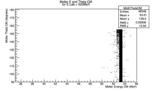
Using the histogram for Theta in the CM frame, we can determine the relative number of events that occur at a given angle. This information will be used to keep the relative number of particles having the same Theta angle, but multiple Psi angles to evenly cover the detector area
Run for Necessary Amount to match Cross Section
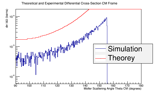
Using the above plot for the target material, we can find the relative amount that each Theta angle should observe for this process which gives a known Moller differential cross section.
| Theta (degrees) | Number of events |
|---|---|
| 90 | 5 |
| 100 | 5 |
| 110 | 6 |
| 120 | 8 |
| 130 | 12 |
| 135 | 20 |
| 140 | 28 |
| 142 | 30 |
| 144 | 40 |
| 146 | 45 |
| 148 | 55 |
| 150 | 70 |
| 152 | 80 |
| 154 | 100 |
We can set up conditional statements to check what range the Theta angle falls in, then by dividing
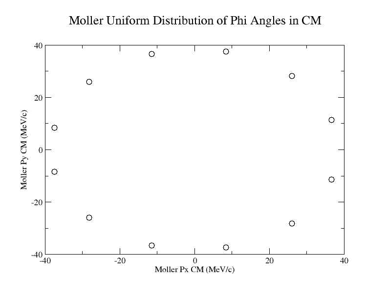
we should find the change in phi needed to give an evenly distributed distribution around the xy plane for a given Theta angle.
Alter Phi Angles
From a C++ program, random Energies and Angle Theta are read from the 2-D histogram created above. Using Relativistic kinematics for CM frame, a 4-momenta vector for the Moller electron is created. Using the properties of the CM frame, a 4-momenta vector for the scattered electron is created. Using the relative counts for number of events at a given angle theta in the CM frame, multiple copies of the Moller CM 4-momenta vector are created. Since the rotation of the angle Phi does not alter the z or total momentum, the same paired version of the scattered electron 4-momenta vector are transfered over from the Moller. Altering Phi Angles
Using two paired 4-momenta vectors in the CM frame, we can rotate them from the "CM-final" state to the "CM-initial" state by having the total momentum of each vector being held only in the z-component as would be expected for two colliding particles (). From this, a Lorentz boost can be performed to find the 4-vectors in the Lab frame for an incoming electron or various energies striking a stationary electron. With the boost vector a second Lorentz boost can be performed from the Final CM Frame to the Final Lab Frame. In this state, the phi distribution is unaffected by the Lorentz boost (perpendicular to direction of relativistic motion), while the theta angle is transformed.
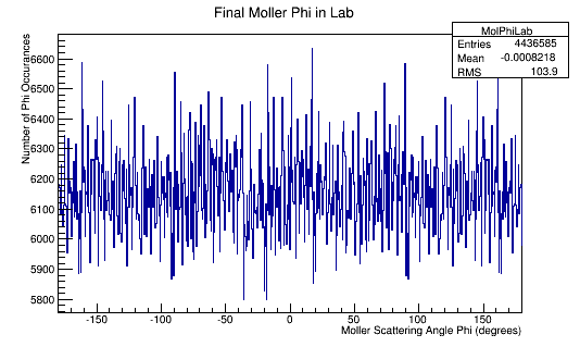
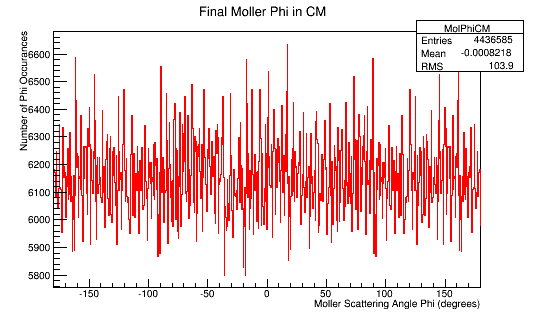
10 separate trials were run for 10,000 events each. The histograms of Momentum, Angle Theta and Phi for the scattered and Moller electron in both the final lab frame and final CM frame were combined using:
hadd -f Total_MakeCM_4e9.root set1/MakeCM_4e9.root set2/MakeCM_4e9.root set3/MakeCM_4e9.root set4/MakeCM_4e9.root set5/MakeCM_4e9.root set6/MakeCM_4e9.root set7/MakeCM_4e9.root set8/MakeCM_4e9.root set9/MakeCM_4e9.root set10/MakeCM_4e9.root
The Phi distribution for the CM and Lab frame.
Their LUND files were combined using
cat set1/Extra_Phi.LUND set2/Extra_Phi.LUND set3/Extra_Phi.LUND set4/Extra_Phi.LUND set5/Extra_Phi.LUND set6/Extra_Phi.LUND set7/Extra_Phi.LUND set8/Extra_Phi.LUND set9/Extra_Phi.LUND set10/Extra_Phi.LUND >Total_Extra_Phi.LUND
resulting in a LUND file that was 13309755 lines in length, which equates to 4436585 entries. This was divided into 177 file parts of 75000 each. The first set from the original data set is shown below.
split -a 4 -d -l 75000 Total_Extra_Phi.LUND Phi_Parts_

It was shown earlier that the differential cross section scale is
For an Ammonia target:
If the beam had 4E9 incident electrons, the differential cross-section would be found with,
Since extra Phi angles have been produced obviously a larger number of incident electrons would be needed. Looking at the number Moller events are created for 1E6, 1E7, and 4E9 incident electrons, we can estimate the number of incident electrons needed for the number of extra Phi angles produced.
| # of Incident Electrons | # of Moller Events | # of E>500MeV |
|---|---|---|
| 1e6 | 38343 | 134 |
| 1e7 | 383633 | 1490 |
| 4e9 | 12444898 | 48548 |
This shows a trait of providing around 100 Moller electrons of Energy greater that 500 MeV for about 1 million incident electrons of Energy 11 GeV. Since the boosting of the number of Phi angles leaves around 4431573 Moller electrons with Energy greater than 500 MeV, this would imply around 4e10 incident electrons of Energy 11 GeV.
Using the same expression, but this time for 4e10 incident electrons,
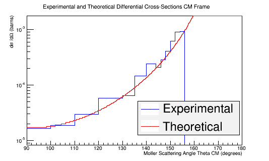
Rebining the histogram to account for the unequal weighting of the bins outlined in the table above
TH1F *Combo=new TH1F("TheoryExperiment","Theoretical and Experimental Differential Cross-Section CM Frame",360,90,180);
Combo->Add(MolThetaCM,8.87e-10);
Combo->Draw();
Double_t Bins[16]={90,100,110,120,130,135,140,142,144,146,148,150,152,154,156,180};
hnew=Combo->Rebin(15,"hnew",Bins);
hnew->Draw();
Theory->Draw("same");
Running LUND files in GEMC
Since the LUND file is limited to 75000 lines, the gemc will have to be run in batch mode;
Creating a batch directory, with two subdirectories; 1)Phi_Parts, 2)submit.
1)Once the LUND file is broken into 178 parts, they can have the LUND extension added by:
prename 's/(Phi_Parts_\d{4})/$1.LUND/' Phi_Parts_*
Placing each of these files into its own directory, within a directory named Phi_Parts
find . -name "*.LUND" -exec sh -c 'mkdir "${1%.*}" ; mv "$1" "${1%.*}" ' _ {} \;
2)Creating the submit directory, and using a c++ program, creating the needed 178
#include <iomanip>
#include <sstream>
#include <iostream>
#include <fstream>

using namespace std;

void submit() {

        for(int a=0;a<2;a++)
        {
                for(int b=0;b<10;b++)
                {
                        for(int c=0;c<10;c++)
                        {
                                string filename="submit0";
                                stringstream hundreds;
                                        hundreds << a;
                                stringstream tens;
                                        tens << b;
                                stringstream ones;
                                        ones << c;
                                string fullname="";
                                fullname=filename + hundreds.str() + tens.str() + ones.str();
                        //              cout << fullname << "\n";

                                ofstream myfile;
                                myfile.open(fullname.c_str());


                                myfile << "#!/bin/sh\n";
                                myfile << "#PBS -l nodes=1\n";
                                myfile << "#PBS -A FIAC\n";
                                myfile << "#PBS -M vanwdani@isu.edu\n";
                                myfile << "#PBS -m abe\n";
                                myfile << "#\n";
                                myfile << "cd /home/lds/src/CLAS/GEMC\n";
                                myfile << "tcsh\n";
                                myfile << "source setup\n";
                                myfile << "cd /home/lds/src/GEANT/geant4.9.6/geant4.9.6-install/bin/geant4.sh\n";
                                myfile << "cd /home/vanwdani/src/GEANT4/geant4.9.6/Simulations/Research/Moller/batch/Phi_Parts/Phi_Parts_0";
                                        myfile <<a<<b<<c<<"\n";
                                myfile << "gemc -USE_GUI=0 -Hall_Material=\"Vacuum\" -INPUT_GEN_FILE=\"LUND, Phi_Parts_0";
                                        myfile <<a<<b<<c;
                                        myfile << ".LUND\" -N=75000 eg12.gcard\n";
                                myfile << "~/src/CLAS/coatjava-1.0/bin/clas12-reconstruction -i eg12.ev -config DCHB::torus=1.0 ";
                                        myfile << "-config DCHB::solenoid=0.0 -config DCTB::kalman=true -o eg12_rec.ev  -s DCHB:DCTB:EC:FTOF:EB\n";
                                myfile << "~/src/CLAS/coatjava-1.0/bin/rungroovy Analysis.groovy eg12_rec.0.evio\n";


                                myfile.close();
                        }
                }
        }

}
This creates the submitXXXX file
#!/bin/sh
#PBS -l nodes=1
#PBS -A FIAC
#PBS -M vanwdani@isu.edu
#PBS -m abe
#
cd /home/lds/src/CLAS/GEMC
tcsh
source setup
cd /home/lds/src/GEANT/geant4.9.6/geant4.9.6-install/bin/geant4.sh
cd /home/vanwdani/src/GEANT4/geant4.9.6/Simulations/Research/Moller/batch/Phi_Parts/Phi_Parts_0000
gemc -USE_GUI=0 -Hall_Material="Vacuum" -INPUT_GEN_FILE="LUND, Phi_Parts_0000.LUND" -N=75000 eg12.gcard
~/src/CLAS/coatjava-1.0/bin/clas12-reconstruction -i eg12.ev -config DCHB::torus=1.0 -config DCHB::solenoid=0.0 -config DCTB::kalman=true -o eg12_rec.ev  -s DCHB:DCTB:EC:FTOF:EB
~/src/CLAS/coatjava-1.0/bin/rungroovy Analysis.groovy eg12_rec.0.evio
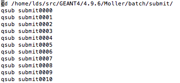
Creating a file named lds-submit
Differential Cross Section
Variables used in Elastic Scattering
Variables Used in Elastic Scattering
