Parent Distribution
Let [math]x_i[/math] represent our ith attempt to measurement the quantity [math]x[/math]
Due to the random errors present in any experiment we should not expect [math]x_i = x[/math].
If we neglect systematic errors, then we should expect [math] x_i[/math] to, on average, follow some probability distribution around the correct value [math]x[/math].
This probability distribution can be referred to as the "parent population".
Average and Variance
Average
The word "average" is used to describe a property of a "parent" probability distribution or a set of observations/measurements made in an experiment which gives an indication of a likely outcome of an experiment.
The symbol
- [math]\mu[/math]
is usually used to represent the "mean" of a known probability (parent) distribution (parent mean) while the "average" of a set of observations/measurements is denoted as
- [math]\bar{x}[/math]
and is commonly referred to as the "sample" average or "sample mean".
Definition of the mean
- [math]\mu \equiv \lim_{N\rightarrow \infty} \frac{\sum x_i}{N}[/math]
Here the above average of a parent distribution is defined in terms of an infinite sum of observations (x_i) of an observable x divided by the number of observations.
[math]\bar{x}[/math] is a calculation of the mean using a finite number of observations
- [math] \bar{x} \equiv \frac{\sum x_i}{N}[/math]
This definition uses the assumption that the result of an experiment, measuring a sample average of [math](\bar{x})[/math], asymptotically approaches the "true" average of the parent distribution [math]\mu[/math] .
Variance
The word "variance" is used to describe a property of a probability distribution or a set of observations/measurements made in an experiment which gives an indication how much an observation will deviate from and average value.
A deviation [math](d_i)[/math] of any measurement [math](x_i)[/math] from a parent distribution with a mean [math]\mu[/math] can be defined as
- [math]d_i\equiv x_i - \mu[/math]
the deviations should average to ZERO for an infinite number of observations by definition of the mean.
Definition of the average
- [math]\mu \equiv \lim_{N\rightarrow \infty} \frac{\sum x_i}{N}[/math]
- [math]\lim_{N\rightarrow \infty} \frac{\sum (x_i - \mu)}{N}[/math]
- [math]= \left ( \lim_{N\rightarrow \infty} \frac{\sum (x_i }{N}\right ) - \mu[/math]
- [math]= \left ( \lim_{N\rightarrow \infty} \frac{\sum (x_i }{N}\right ) - \lim_{N\rightarrow \infty} \frac{\sum x_i}{N} = 0[/math]
But the AVERAGE DEVIATION [math](\bar{d})[/math] is given by an average of the magnitude of the deviations given by
- [math]\bar{d} = \lim_{N\rightarrow \infty} \frac{\sum \left | (x_i - \mu)\right |}{N}[/math] = a measure of the dispersion of the expected observations about the mean
Taking the absolute value though is cumbersome when performing a statistical analysis so one may express this dispersion in terms of the variance
A typical variable used to denote the variance is
- [math]\sigma^2[/math]
and is defined as
- [math]\sigma^2 = \lim_{N\rightarrow \infty}\left [ \frac{\sum (x_i-\mu)^2 }{N}\right ][/math]
Standard Deviation
The standard deviation is defined as the square root of the variance
- S.D. = [math]\sqrt{\sigma^2}[/math]
The mean should be thought of as a parameter which characterizes the observations we are making in an experiment. In general the mean specifies the probability distribution that is representative of the observable we are trying to measure through experimentation.
The variance characterizes the uncertainty associated with our experimental attempts to determine the "true" value. Although the mean and true value may not be equal, their difference should be less than the uncertainty given by the governing probability distribution.
Another Expression for Variance
Using the definition of variance (omitting the limit as [math]n \rightarrow \infty[/math])
- Evaluating the definition of variance
- [math]\sigma^2 \equiv \frac{\sum(x_i-\mu)^2}{N} = \frac{\sum (x_i^2 -2x_i \mu + \mu^2)}{N} = \frac{\sum x_i^2}{N} - 2 \mu \frac{\sum x_i}{N} + \frac{N \mu^2}{N} [/math]
- [math] = \frac{\sum x_i^2}{N} -2 \mu^2 + \mu^2 =\frac{\sum x_i^2}{N} - \mu^2[/math]
- [math]\frac{\sum(x_i-\mu)^2}{N} =\frac{\sum x_i^2}{N} - \mu^2[/math]
You can recast the above in terms of expectation value where
[math]E[x] \equiv \sum x_i P_x(x)[/math]
- [math]\Rightarrow \sigma^2 = E[(x-\mu)^2] = \sum_{x=0}^n (x_i - \mu)^2 P(x_i)[/math]
- [math]= E[x^2] - \left ( E[x]\right )^2 = \sum_{x=0}^n x_i^2 P(x_i) - \left ( \sum_{x=0}^n x_i P(x_i)\right )^2[/math]
Average for an unknown probability distribution (parent population)
If the "Parent Population" is not known, you are just given a list of numbers with no indication of the probability distribution that they were drawn from, then the average and variance may be calculate as shown below.
Arithmetic Mean and variance
If [math]n[/math] observables are mode in an experiment then the arithmetic mean of those observables is defined as
- [math]\bar{x} = \frac{\sum_{i=1}^{i=N} x_i}{N}[/math]
The "unbiased" variance of the above sample is defined as
- [math]s^2 = \frac{\sum_{i=1}^{i=N} (x_i - \bar{x})^2}{N-1}[/math]
- If you were told that the average is [math]\bar{x}[/math] then you can calculate the
"true" variance of the above sample as
- [math]\sigma^2 = \frac{\sum_{i=1}^{i=N} (x_i - \bar{x})^2}{N}[/math] = RMS Error= Root Mean Squared Error
- Note
- RMS = Root Mean Square = [math]\frac{\sum_i^n x_i^2}{N}[/math] =
Statistical Variance decreases with N
The repetition of an experiment can decrease the STATISTICAL error of the experiment
Consider the following:
The average value of the mean of a sample of n observations drawn from the parent population is the same as the average value of each observation. (The average of the averages is the same as one of the averages)
- [math]\bar{x} = \frac{\sum x_i}{N} =[/math] sample mean
- [math]\overline{\left ( \bar{x} \right ) } = \frac{\sum{\bar{x}_i}}{N} =\frac{1}{N} N \bar{x_i} = \bar{x}[/math] if all means are the same
This is the reason why the sample mean is a measure of the population average ( [math]\bar{x} \sim \mu[/math])
Now consider the variance of the average of the averages (this is not the variance of the individual measurements but the variance of their means)
- [math]\sigma^2_{\bar{x}} = \frac{\sum \left (\bar{x} -\overline{\left ( \bar{x} \right ) } \right )^2}{N} =\frac{\sum \bar{x_i}^2}{N} -\left( \overline{\left ( \bar{x} \right ) } \right )^2[/math]
- [math]=\frac{\sum \bar{x_i}^2}{N} -\left( \bar{x} \right )^2[/math]
- [math]=\frac{\sum \left( \sum \frac{x_i}{N}\right)^2}{N} -\left( \bar{x} \right )^2[/math]
- [math]=\frac{1}{N^2}\frac{\sum \left( \sum x_i\right)^2}{N} -\left( \bar{x} \right )^2[/math]
- [math]=\frac{1}{N^2}\frac{\sum \left (\sum x_i^2 + \sum_{i \ne j} x_ix_j \right )}{N} -\left( \bar{x} \right )^2[/math]
- [math]=\frac{1}{N^2} \left [ \frac{\sum \left(\sum x_i^2 \right)}{N} + \frac{ \sum \left (\sum_{i \ne j} x_ix_j \right )}{N} \right ] -\left( \bar{x} \right )^2[/math]
- If the measurements are all independent
- Then [math] \frac{\sum_{i \ne j} x_i x_j}{N} = \frac{\sum x_i}{N} \frac{ \sum x_j}{N}[/math] : if [math]x_i[/math] is independent of [math]x_j[/math] ([math]i \ne j[/math])
- [math]= \left ( \frac{\sum x_i}{N} \right)^2 = \bar{x}^2[/math]
example:
- (x_1x_2 + x_1x_3 + x_2x_1+x_2x_3+x_3x_1+x_3x_2+ ...) = (x_1+x_2+x_3)
The above part of the proof needs work
- [math]\sigma^2_{\bar{x}}=\frac{1}{N^2} \left [ \frac{\sum \left(\sum x_i^2 \right)}{N} + \sum_{i \ne j} \bar{x}^2 \right ] -\left( \bar{x} \right )^2[/math]
I use the expression [math]\sigma^2 = E[x^2] - \left ( E[x] \right)^2[/math] again, except for[math] x_i[/math] and not [math]\bar{x}[/math] and turn it around so
- [math]\frac{\left(\sum x_i^2 \right)}{N} = \sigma^2 + \left ( \frac{\sum x_i}{N}\right)^2[/math]
Now I have
- [math]\sigma^2_{\bar{x}}=\frac{1}{N^2} \left [ \sum \left (\sigma^2 + \left ( \frac{\sum x_i}{N} \right )^2 \right )+ \sum_{i \ne j} \bar{x}^2 \right ] -\left( \bar{x} \right )^2[/math]
- [math]=\frac{1}{N^2} \left [ N\sigma^2 + N\left ( \frac{\sum x_i}{N} \right )^2 + \sum_{i \ne j} \bar{x}^2 \right ] -\left( \bar{x} \right )^2[/math]
- [math]=\frac{1}{N^2} \left [ N\sigma^2 + N\left ( \frac{\sum x_i}{N} \right )^2 + N(N-1) \bar{x}^2 \right ] -\left( \bar{x} \right )^2[/math] Number of cross terms is N*(N-1)
- [math]=\frac{1}{N^2} \left [ N\sigma^2 + N\left ( \frac{\sum x_i}{N} \right )^2 + (N^2 -N) \left ( \frac{\sum x_i}{N} \right )^2 \right ] -\left( \bar{x} \right )^2[/math] Number of cross terms is N*(N-1)
- [math]= \left [ \frac{\sigma^2}{N} + \left ( \frac{\sum x_i}{N} \right )^2 \right ] -\left( \bar{x} \right )^2[/math]
- [math]= \left [ \frac{\sigma^2}{N} + \left ( \bar{x}\right )^2 \right ] -\left( \bar{x} \right )^2[/math]
- [math]= \frac{\sigma^2}{N} [/math]
The above is the essence of counting statistics.
It says that the STATISTICAL error in an experiment decreases as a function of [math]\frac{1}{\sqrt N}[/math]
Biased and Unbiased variance
Where does this idea of an unbiased variance come from?
Using the same procedure as the previous section let's look at the average variance of the variances.
A sample variance of [math]n[/math] measurements of [math]x_i[/math] is
- [math]\sigma_n^2 = \frac{\sum(x_i-\bar{x})^2}{n} = E[x^2] - \left ( E[x] \right)^2 = \frac{\sum x_i^2}{n} -\left ( \bar{x} \right)^2[/math]
To determine the "true" variance consider taking average of several sample variances (this is the same argument used above which let to [math]\overline{(\bar{x})} = \bar{x}[/math] )
- [math]\frac{\sum_j \left [ \sigma_n^2 \right ]_j}{N} = \frac{ \sum_j \left [ \frac{\sum_i x_i^2}{n} -\left ( \bar{x} \right)^2 \right ]_j}{N}[/math]
- [math]= \frac{1}{n}\sum_i \left ( \frac{\sum_j x_j^2}{N} \right )_i - \frac {\sum_j \left ( \bar{x} \right)^2 }{N}[/math]
- [math]= \frac{1}{n}\sum_i \left ( \frac{\sum_j x_j^2}{N} \right )_i - \left [ \left ( \frac {\sum_j \bar{x}}{N} \right)^2 + \sigma_{\bar{x}}^2\right ][/math] : as shown previously [math]E[\bar{x}^2] = \left ( E[\bar{x}] \right )^2 + \sigma_{\bar{x}}^2[/math]
- [math]= \frac{1}{n}\sum_i \left ( \left [ \left (\frac{\sum_j x_j}{N}\right)^2 + \sigma^2 \right ]\right )_i - \left [ \left ( \frac {\sum_j x_j}{N} \right)^2 + \frac{\sigma^2}{n}\right ][/math] : also shown previously[math]\overline{\left ( \bar{x} \right ) } = \bar{x}[/math] the universe average is the same as the sample average
- [math]= \frac{1}{n} \left ( n\left [ \left (\frac{\sum_j x_j}{N}\right)^2 + n\sigma^2 \right ]\right )_i - \left [ \left ( \frac {\sum_j x_j}{N} \right)^2 + \frac{\sigma^2}{n}\right ][/math]
- [math]= \sigma^2 - \frac{\sigma^2}{n}[/math]
- [math]= \frac{n-1}{n}\sigma^2[/math]
- [math]\Rightarrow \sigma^2 = \frac{n}{n-1}\frac{\sum \sigma_i^2}{N}[/math]
Here
- [math]\sigma^2 =[/math] the sample variance
- [math]\frac{\sum \sigma_i^2}{N} =[/math] an average of all possible sample variance which should be equivalent to the "true" population variance.
- [math]\Rightarrow \frac{\sum \sigma_i^2}{N} \sim \sum \frac{x_i-\bar{x}}{n}[/math] : if all the variances are the same this would be equivalent
- [math]\sigma^2 = \frac{n}{n-1}\frac{\sum(x_i-\bar{x})}{n}[/math]
- [math]= \frac{\sum(x_i-\bar{x})}{n-1} =[/math] unbiased sample variance
Probability Distributions
Mean(Expectation value) and variance
Mean of Discrete Probability Distribution
In the case that you know the probability distribution you can calculate the mean[math] (\mu)[/math] or expectation value E(x) and standard deviation as
For a Discrete probability distribution
[math]\mu = E[x]=\lim_{N \rightarrow \infty} \frac{\sum_{i=1}^n x_i P(x_i)}{N}[/math]
where
[math]N=[/math] number of observations
[math]n=[/math] number of different possible observable variables
[math]x_i =[/math] ith observable quantity
[math]P(x_i) =[/math] probability of observing [math]x_i[/math] = Probability Mass Distribution for a discrete probability distribution
Mean of a continuous probability distibution
The average (mean) of a sample drawn from any probability distribution is defined in terms of the expectation value E(x) such that
The expectation value for a continuous probability distribution is calculated as
- [math]\mu = E(x) = \int_{-\infty}^{\infty} x P(x)dx[/math]
Variance
Variance of a discrete PDF
[math]\sigma^2 = \sum_{i=1}^n \left [ (x_i - \mu)^2 P(x_i)\right ][/math]
Variance of a Continuous PDF
[math]\sigma^2 = \int_{-\infty}^{\infty} \left [ (x - \mu)^2 P(x)\right ]dx[/math]
Expectation of Arbitrary function
If [math]f(x)[/math] is an arbitrary function of a variable [math]x[/math] governed by a probability distribution [math]P(x)[/math]
then the expectation value of [math]f(x)[/math] is
[math]E[f(x)] = \sum_{i=1}^N f(x_i) P(x_i) [/math]
or if a continuous distribtion
[math]E[f(x)] = \int_{-\infty}^{\infty} f(x) P(x)dx[/math]
Uniform
The Uniform probability distribution function is a continuous probability function over a specified interval in which any value within the interval has the same probability of occurring.
Mathematically the uniform distribution over an interval from a to b is given by
- [math]P_U(x) =\left \{ {\frac{1}{b-a} \;\;\;\; x \gt a \mbox{ and } x \lt b \atop 0 \;\;\;\; x\gt b \mbox{ or } x \lt a} \right .[/math]
Mean of Uniform PDF
- [math]\mu = \int_{-\infty}^{\infty} xP_U(x)dx = \int_{a}^{b} \frac{x}{b-a} dx = \left . \frac{x^2}{2(b-a)} \right |_a^b = \frac{1}{2}\frac{b^2 - a^2}{b-a} = \frac{1}{2}(b+a)[/math]
Variance of Uniform PDF
- [math]\sigma^2 = \int_{-\infty}^{\infty} (x-\mu)^2 P_U(x)dx = \int_{a}^{b} \frac{\left (x-\frac{b+a}{2}\right )^2}{b-a} dx = \left . \frac{(x -\frac{b+a}{2})^3}{3(b-a)} \right |_a^b [/math]
- [math]=\frac{1}{3(b-a)}\left [ \left (b -\frac{b+a}{2} \right )^3 - \left (a -\frac{b+a}{2} \right)^3\right ][/math]
- [math]=\frac{1}{3(b-a)}\left [ \left (\frac{b-a}{2} \right )^3 - \left (\frac{a-b}{2} \right)^3\right ][/math]
- [math]=\frac{1}{24(b-a)}\left [ (b-a)^3 - (-1)^3 (b-a)^3\right ][/math]
- [math]=\frac{1}{12}(b-a)^2[/math]
Now use ROOT to generate uniform distributions.
http://wiki.iac.isu.edu/index.php/TF_ErrAna_InClassLab#Day_3
Binomial Distribution
Binomial random variable describes experiments in which the outcome has only 2 possibilities. The two possible outcomes can be labeled as "success" or "failure". The probabilities may be defined as
- p
- the probability of a success
and
- q
- the probability of a failure.
If we let [math]X[/math] represent the number of successes after repeating the experiment [math]n[/math] times
Experiments with [math]n=1[/math] are also known as Bernoulli trails.
Then [math]X[/math] is the Binomial random variable with parameters [math]n[/math] and [math]p[/math].
The number of ways in which the [math]x[/math] successful outcomes can be organized in [math]n[/math] repeated trials is
- [math]\frac{n !}{ \left [ (n-x) ! x !\right ]}[/math] where the [math] ![/math] denotes a factorial such that [math]5! = 5\times4\times3\times2\times1[/math].
The expression is known as the binomial coefficient and is represented as
[math]{n\choose x}=\frac{n!}{x!(n-x)!}[/math]
The probability of any one ordering of the success and failures is given by
[math]P( \mbox{experimental ordering}) = p^{x}q^{n-x}[/math]
This means the probability of getting exactly k successes after n trials is
- [math]P_B(x) = {n\choose x}p^{x}q^{n-x} [/math]
Mean
It can be shown that the Expectation Value of the distribution is
- [math]\mu = n p[/math]
- [math]\mu = \sum_{x=0}^n x P_B(x) = \sum_{x=0}^n x \frac{n!}{x!(n-x)!} p^{x}q^{n-x}[/math]
- [math] = \sum_{x=1}^n \frac{n!}{(x-1)!(n-x)!} p^{x}q^{n-x}[/math] :summation starts from x=1 and not x=0 now
- [math] = np \sum_{x=1}^n \frac{(n-1)!}{(x-1)!(n-x)!} p^{x-1}q^{n-x}[/math] :factor out [math]np[/math] : replace n-1 with m everywhere and it looks like binomial distribution
- [math] = np \sum_{y=0}^{n-1} \frac{(n-1)!}{(y)!(n-y-1)!} p^{y}q^{n-y-1}[/math] :change summation index so y=x-1, now n become n-1
- [math] = np \sum_{y=0}^{n-1} \frac{(n-1)!}{(y)!(n-1-y)!} p^{y}q^{n-1-y}[/math] :
- [math] = np (q+p)^{n-1}[/math] :definition of binomial expansion
- [math] = np 1^{n-1}[/math] :q+p =1
- [math] = np [/math]
variance
- [math]\sigma^2 = npq[/math]
- Remember
- [math]\frac{\sum(x_i-\mu)^2}{N} = \frac{\sum (x_i^2 -2x_i \mu + \mu^2)}{N} = \frac{\sum x_i^2}{N} - 2 \mu \frac{\sum x_i}{N} + \frac{N \mu^2}{N} [/math]
- [math] = \frac{\sum x_i^2}{N} -2 \mu^2 + \mu^2 =\frac{\sum x_i^2}{N} - \mu^2[/math]
- [math]\frac{\sum(x_i-\mu)^2}{N} =\frac{\sum x_i^2}{N} - \mu^2[/math]
- [math]\Rightarrow \sigma^2 = E[(x-\mu)^2] = \sum_{x=0}^n (x_i - \mu)^2 P_B(x_i)[/math]
- [math]= E[x^2] - \left ( E[x]\right )^2 = \sum_{x=0}^n x_i^2 P_B(x_i) - \left ( \sum_{x=0}^n x_i P_B(x_i)\right )^2[/math]
To calculate the variance of the Binomial distribution I will just calculate [math]E[x^2][/math] and then subtract off [math]\left ( E[x]\right )^2[/math].
- [math]E[x^2] = \sum_{x=0}^n x^2 P_B(x)[/math]
- [math]= \sum_{x=1}^n x^2 P_B(x)[/math] : x=0 term is zero so no contribution
- [math]=\sum_{x=1}^n x^2 \frac{n!}{x!(n-x)!} p^{x}q^{n-x}[/math]
- [math]= np \sum_{x=1}^n x \frac{(n-1)!}{(x-1)!(n-x)!} p^{x-1}q^{n-x}[/math]
Let m=n-1 and y=x-1
- [math]= np \sum_{y=0}^n (y+1) \frac{m!}{(y)!(m-1-y+1)!} p^{y}q^{m-1-y+1}[/math]
- [math]= np \sum_{y=0}^n (y+1) P(y)[/math]
- [math]= np \left ( \sum_{y=0}^n y P(y) + \sum_{y=0}^n (1) P(y) \right)[/math]
- [math]= np \left ( mp + 1 \right)[/math]
- [math]= np \left ( (n-1)p + 1 \right)[/math]
- [math]\sigma^2 = E[x^2] - \left ( E[x] \right)^2 = np \left ( (n-1)p + 1 \right) - (np)^2 = np(1-p) = npq[/math]
Examples
The number of times a coin toss is heads.
The probability of a coin landing with the head of the coin facing up is
- [math]P = \frac{\mbox{number of desired outcomes}}{\mbox{number of possible outcomes}} = \frac{1}{2}[/math] = Uniform distribution with a=0 (tails) b=1 (heads).
Suppose you toss a coin 4 times. Here are the possible outcomes
| order Number
|
Trial #
|
# of Heads
|
|
1 |
2 |
3 |
4 |
|
| 1 |
t |
t |
t |
t |
0
|
| 2 |
h |
t |
t |
t |
1
|
| 3 |
t |
h |
t |
t |
1
|
| 4 |
t |
t |
h |
t |
1
|
| 5 |
t |
t |
t |
h |
1
|
| 6 |
h |
h |
t |
t |
2
|
| 7 |
h |
t |
h |
t |
2
|
| 8 |
h |
t |
t |
h |
2
|
| 9 |
t |
h |
h |
t |
2
|
| 10 |
t |
h |
t |
h |
2
|
| 11 |
t |
t |
h |
h |
2
|
| 12 |
t |
h |
h |
h |
3
|
| 13 |
h |
t |
h |
h |
3
|
| 14 |
h |
h |
t |
h |
3
|
| 15 |
h |
h |
h |
t |
3
|
| 16 |
h |
h |
h |
h |
4
|
The probability of order #1 happening is
P( order #1) = [math]\left ( \frac{1}{2} \right )^0\left ( \frac{1}{2} \right )^4 = \frac{1}{16}[/math]
P( order #2) = [math]\left ( \frac{1}{2} \right )^1\left ( \frac{1}{2} \right )^3 = \frac{1}{16}[/math]
The probability of observing the coin land on heads 3 times out of 4 trials is.
[math]P(x=3) = \frac{4}{16} = \frac{1}{4} = {n\choose x}p^{x}q^{n-x} = \frac{4 !}{ \left [ (4-3) ! 3 !\right ]} \left ( \frac{1}{2}\right )^{3}\left ( \frac{1}{2}\right )^{4-3} = \frac{24}{1 \times 6} \frac{1}{16} = \frac{1}{4}[/math]
A 6 sided die
A die is a 6 sided cube with dots on each side. Each side has a unique number of dots with at most 6 dots on any one side.
P=1/6 = probability of landing on any side of the cube.
Expectation value :
- The expected (average) value for rolling a single die.
- [math]E({\rm Roll\ With\ 6\ Sided\ Die}) =\sum_i x_i P(x_i) =1 \left ( \frac{1}{6} \right) + 2\left ( \frac{1}{6} \right)+ 3\left ( \frac{1}{6} \right)+ 4\left ( \frac{1}{6} \right)+ 5\left ( \frac{1}{6} \right)+ 6\left ( \frac{1}{6} \right)=\frac{1 + 2 + 3 + 4 + 5 + 6}{6} = 3.5[/math]
The variance:
- [math]E({\rm Roll\ With\ 6\ Sided\ Die}) =\sum_i (x_i - \mu)^2 P(x_i) [/math]
- [math]= (1-3.5)^2 \left ( \frac{1}{6} \right) + (2-3.5)^2\left ( \frac{1}{6} \right)+ (3-3.5)^2\left ( \frac{1}{6} \right)+ (4-3.5)^2\left ( \frac{1}{6} \right)+ (5-3.5)^2\left ( \frac{1}{6} \right)+ (6-3.5)^2\left ( \frac{1}{6} \right) =2.92[/math]
- [math]= \sum_i (x_i)^2 P(x_i) - \mu^2 = \left [ 1 \left ( \frac{1}{6} \right) + 4\left ( \frac{1}{6} \right)+ 9\left ( \frac{1}{6} \right)+ 16\left ( \frac{1}{6} \right)+ 25\left ( \frac{1}{6} \right)+ 36\left ( \frac{1}{6} \right) \right ] - (3.5)^3 =2.92[/math]
If we roll the die 10 times what is the probability that X dice will show a 6?
A success will be that the die landed with 6 dots face up.
So the probability of this is 1/6 (p=1/6) , we toss it 10 times (n=10) so the binomial distribution function for a success/fail experiment says
[math]P_B(x) = {n\choose x}p^{x}q^{n-x} = \frac{10 !}{ \left [ (10-x) ! x !\right ]} \left ( \frac{1}{6}\right )^{x}\left ( \frac{5}{6}\right )^{10-x} [/math]
So the probability the die will have 6 dots face up in 4/10 rolls is
[math]P_B(x=4) = \frac{10 !}{ \left [ (10-4) ! 4 !\right ]} \left ( \frac{1}{6}\right )^{4}\left ( \frac{5}{6}\right )^{10-4} [/math]
- [math] = \frac{10 !}{ \left [ (6) ! 4 !\right ]} \left ( \frac{1}{6}\right )^{4}\left ( \frac{5}{6}\right )^{6} = \frac{210 \times 5^6}{6^10}=0.054 [/math]
Mean = np =[math]\mu = 10/6 = 1.67[/math]
Variance = [math]\sigma^2 = 10 (1/6)(5/6) = 1.38[/math]
Poisson Distribution
The Poisson distribution is an approximation to the binomial distribution in the event that the probability of a success is quite small [math](p \ll 1)[/math]. As the number of repeated observations (n) gets large, the binomial distribution becomes more difficult to evaluate because of the leading term
- [math]\frac{n !}{ \left [ (n-x) ! x !\right ]}[/math]
The poisson distribution overcomes this problem by defining the probability in terms of the average [math]\mu[/math].
- [math]P_P(x) = \frac{\mu^x e^{-\mu}}{x!}[/math]
Poisson as approximation to Binomial
To drive home the idea that the Poisson distribution approximates a Binomial distribution at small p and large n consider the following derivation
The Binomial Probability Distriubtions is
- [math]P_B(x) = \frac{n!}{x!(n-x)!}p^{x}q^{n-x}[/math]
The term
- [math] \frac{n!}{(n-x)!} = \frac{(n-x)! (n-x+1) (n-x + 2) \dots (n-1)(n)}{(n-x)!}[/math]
- [math]= n (n-1)(n-2) \dots (n-x+2) (n-x+1)[/math]
- IFF [math]x \ll n \Rightarrow[/math] we have x terms above
- then [math]\frac{n!}{(n-x)!} =n^x[/math]
- example:[math] \frac{100!}{(100-1)!} = \frac{99! \times 100}{99!} = 100^1[/math]
This leave us with
- [math]P(x) = \frac{n^x}{x!}p^{x}q^{n-x}= \frac{(np)^x}{x!}(1-p)^{n-x}[/math]
- [math]= \frac{(\mu)^x}{x!}(1-p)^{n}(1-p)^{-x}[/math]
- [math](1-p)^{-x} = \frac{1}{(1-p)^x} = 1+px = 1 : p \ll 1[/math]
- [math]P(x) = \frac{(\mu)^x}{x!}(1-p)^{n}[/math]
- [math](1-p)^{n} = \left [(1-p)^{1/p} \right]^{\mu}[/math]
- [math]\lim_{p \rightarrow 0} \left [(1-p)^{1/p} \right]^{\mu} = \left ( \frac{1}{e} \right)^{\mu} = e^{- \mu}[/math]
- For [math]x \ll n[/math]
- [math]\lim_{p \rightarrow 0}P_B(x,n,p ) = P_P(x,\mu)[/math]
Derivation of Poisson Distribution
The mean free path of a particle traversing a volume of material is a common problem in nuclear and particle physics. If you want to shield your apparatus or yourself from radiation you want to know how far the radiation travels through material.
The mean free path is the average distance a particle travels through a material before interacting with the material.
- If we let [math]\lambda[/math] represent the mean free path
- Then the probability of having an interaction after a distance x is
- [math]\frac{x}{\lambda}[/math]
as a result
- [math]1-\frac{x}{\lambda}= P(0,x, \lambda)[/math] = probability of getting no events after a length dx
When we consider [math]\frac{x}{\lambda} \ll 1[/math] ( we are looking for small distances such that the probability of no interactions is high)
- [math]P(0,x, \lambda) = e^{\frac{-x}{\lambda}} \approx 1 - \frac{x}{\lambda}[/math]
Now we wish to find the probability of finding [math]N[/math] events over a distance [math]x[/math] given the mean free path.
This is calculated as a joint probability. If it were the case that we wanted to know the probability of only one interaction over a distance [math]L[/math]. Then we would want to multiply the probability that an interaction happened after a distance [math]dx[/math] by the probability that no more interactions happen by the time the particle reaches the distance [math]L[/math].
For the case of [math]N[/math] interactions, we have a series of [math]N[/math] interactions happening over N intervals of [math]dx[/math] with the probability [math]dx/\lambda[/math]
- [math]P(N,x,\lambda)[/math] = probability of finding [math]N[/math] events within the length [math]x[/math]
- [math]= \frac{dx_1}{\lambda}\frac{dx_2}{\lambda}\frac{dx_3}{\lambda} \dots \frac{dx_N}{\lambda} e^{\frac{-x}{\lambda}}[/math]
The above expression represents the probability for a particular sequence of events in which an interaction occurs after a distance [math]dx_1[/math] then a interaction after [math]dx_2[/math] , [math]\dots[/math]
So in essence the above expression is a "probability element" where another probability element may be
- [math] P(N,x, \lambda)=\frac{dx_2}{\lambda}\frac{dx_1}{\lambda}\frac{dx_3}{\lambda} \dots \frac{dx_N}{\lambda} e^{\frac{-x}{\lambda}}[/math]
where the first interaction occurs after the distance [math]x_2[/math].
- [math]= \Pi_{i=1}^{N} \left [ \frac{dx_i}{\lambda} \right ] e^{\frac{-x}{\lambda}}[/math]
So we can write a differential probability element which we need to add up as
- [math]d^NP(N,x, \lambda)=\frac{1}{N!} \Pi_{i=1}^{N} \left [ \frac{dx_i}{\lambda} \right ] e^{\frac{-x}{\lambda}}[/math]
The N! accounts for the degeneracy in which for every N! permutations there is really only one new combination. ie we are double counting when we integrate.
Using the integral formula
- [math] \Pi_{i=1}^{N} \left [\int_0^x \frac{dx_i}{\lambda} \right ]= \left [ \frac{x}{\lambda}\right]^N[/math]
we end up with
[math]P(N,x, \lambda) = \frac{\left [ \frac{x}{\lambda}\right]^N}{N!} e^{\frac{-x}{\lambda}}[/math]
Mean of Poisson Dist
- [math]\mu = \sum_{i=1}^{\infty} i P(i,x, \lambda)[/math]
- [math]= \sum_{i=1}^{\infty} i \frac{\left [ \frac{x}{\lambda}\right]^i}{i!} e^{\frac{-x}{\lambda}}
= \frac{x}{\lambda} \sum_{i=1}^{\infty} \frac{\left [ \frac{x}{\lambda}\right]^{(i-1)}}{(i-1)!} e^{\frac{-x}{\lambda}} = \frac{x}{\lambda}
[/math]
- [math]P_P(x,\mu) = \frac{\mu^x e^{-\mu}}{x!} [/math]
Variance of Poisson Dist
For Homework you will show, in a manner similar to the above mean calculation, that the variance of the Poisson distribution is
- [math]\sigma^2 = \mu[/math]
Gaussian
The Gaussian (Normal) distribution is an approximation of the Binomial distribution for the case of a large number of possible different observations. Poisson approximated the binomial distribution for the case when p<<1 ( the average number of successes is a lot smaller than the number of trials [math](\mu = np)[/math] ).
The Gaussian distribution is accepted as one of the most likely distributions to describe measurements.
A Gaussian distribution which is normalized such that its integral is unity is refered to as the Normal distribution. You could mathematically construct a Gaussian distribution which is not normalized to unity (this is often done when fitting experimental data).
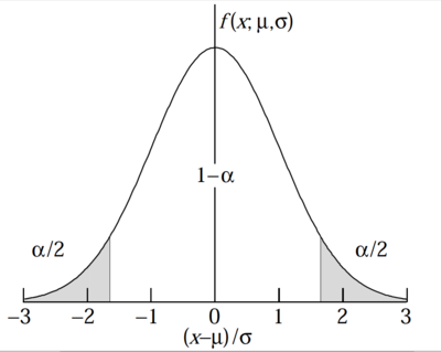
- [math]P_G(x,\mu, \sigma) = \frac{1}{\sigma \sqrt{2 \pi}}e^{-\frac{1}{2} \left( \frac{x -\mu}{\sigma} \right) ^2}[/math] = probability of observing [math]x[/math] from a Gaussian parent distribution with a mean [math]\mu[/math] and standard deviation [math]\sigma[/math].
Half-Width [math]\Gamma[/math] (a.k.a. Full Width as Half Max)
The half width [math]\Gamma[/math] is used to describe the range of [math]x[/math] through which the distributions amplitude decreases to half of its maximum value.
- ie
- [math]P_G(\mu \pm \frac{\Gamma}{2}, \mu, \sigma) = \frac{P_G(\mu,\mu,\sigma)}{2}[/math]
- Side note
- the point of steepest descent is located at [math]x \pm \sigma[/math] such that
- [math]P_G(\mu \pm \sigma, \mu, \sigma) = e^{1/2} P_G(\mu,\mu,\sigma)[/math]
Probable Error (P.E.)
The probable error is the range of [math]x[/math] in which half of the observations (values of [math]x[/math]) are expected to fall.
- [math]x= \mu \pm P.E.[/math]
Binomial with Large N becomes Gaussian
Consider the binomial distribution in which a fair coin is tossed a large number of times (N is very large and an EVEN number N=2n)
What is the probability you get exactly [math]\frac{1}{2}N -s[/math] heads and [math]\frac{1}{2}N +s[/math] tails where s is an integer?
The Binomial Probability distribution is given as
- [math]P_B(x) = {N\choose x}p^{x}q^{N-x} = \frac{N!}{x!(N-x)!}p^{x}q^{N-x}[/math]
p = probability of success= 1/2
q= 1-p = 1/2
N = number of trials =2n
x= number of successes=n-s
- [math]P_B(n-s) = \frac{2n!}{(n-s)!(2n-n+s)!}p^{n-s}q^{2n-n+s}[/math]
- [math]= \frac{2n!}{(n-s)!(n+s)!}p^{n-s}q^{n+s}[/math]
- [math]= \frac{2n!}{(n-s)!(n+s)!} \left(\frac{1}{2}\right)^{n-s} \left(\frac{1}{2}\right)^{n+s}[/math]
- [math]= \frac{2n!}{(n-s)!(n+s)!} \left(\frac{1}{2}\right)^{2n}[/math]
Now let's cast this probability with respect to the probability that we get an even number of heads and tails by defining the following ratio R such that
- [math]R \equiv \frac{P_B(n-s)}{P_B(n)}[/math]
- [math]P_B(x=n) = \frac{N!}{n!(N-n)!}p^{n}q^{N-n} = \frac{(2n)!}{n!(n)!}p^{n}q^{n} = \frac{(2n)!}{(n)!(n)!} \left(\frac{1}{2}\right)^{2n}[/math]
- [math]R = \frac{\frac{2n!}{(n-s)!(n+s)!} \left(\frac{1}{2}\right)^{2n}}{\frac{(2n)!}{(n)!(n)!} \left(\frac{1}{2}\right)^{2n}} = \frac{n! n!}{(n-s)! (n+s)!}[/math]
Take the natural logarithm of both sides
- [math] \ln (R) = \ln \left ( \frac{n! n!}{(n-s)! (n+s)!} \right) = \ln(n!)+\ln(n!) - \ln\left[(n-s)!\right ] - \ln \left[(n+s)!\right] = 2 \ln(n!) - \ln\left [ (n-s)! \right ] - \ln \left [ (n+s)! \right ][/math]
Stirling's Approximation says
- [math]n! \sim \left (2 \pi n\right)^{1/2} n^n e^{-n}[/math]
- [math]\Rightarrow [/math]
- [math]\ln(n!) \sim \ln \left [ \left (2 \pi n\right)^{1/2} n^n e^{-n}\right ] = \ln \left [ \left (2 \pi \right)^{1/2} \right ] +\ln \left [ n^{1/2} \right ] +\ln\left [ n^n \right ] + \ln \left [e^{-n}\right ][/math]
- [math]= \ln \left [ \left (2 \pi \right)^{1/2} \right ] +\ln \left [ n^{1/2} \right ] +n\ln\left [ n \right ] + (-n)[/math]
- [math]= \ln \left [ \left (2 \pi \right)^{1/2} \right ] +\ln \left [ n^{1/2} \right ] +n(\ln\left [ n \right ] -1 )[/math]
similarly
- [math]\ln\left [(n-s)! \right ] \sim \ln \left [ \left (2 \pi \right)^{1/2} \right ] +\ln \left [ (n-1)^{1/2} \right ] + (n-s)(\ln\left [ (n-s) \right ] -1 )[/math]
- [math]\ln\left [(n+s)! \right ] \sim \ln \left [ \left (2 \pi \right)^{1/2} \right ] +\ln \left [ (n+1)^{1/2} \right ] + (n+s)(\ln\left [ (n+s) \right ] -1 )[/math]
- [math]\Rightarrow \ln (R) = 2 \times \left (\ln \left [ \left (2 \pi \right)^{1/2} \right ] +\ln \left [ n^{1/2} \right ] +n(\ln\left [ n \right ] -1 ) \right ) [/math]
- [math]- \left ( \ln \left [ \left (2 \pi \right)^{1/2} \right ] +\ln \left [ (n-1)^{1/2} \right ] + (n-s)(\ln\left [ (n-s) \right ] -1 )\right )[/math]
- [math] -\left ( \ln \left [ \left (2 \pi \right)^{1/2} \right ] +\ln \left [ (n+1)^{1/2} \right ] + (n+s)(\ln\left [ (n+s) \right ] -1 )\right ) [/math]
- [math]= 2 \ln \left [ n^{1/2} \right ] +2 n(\ln\left [ n \right ] -1 ) - \ln \left [ (n-1)^{1/2} \right ] - (n-s)(\ln\left [ (n-s) \right ] -1 ) -\ln \left [ (n+1)^{1/2} \right ] - (n+s)(\ln\left [ (n+s) \right ] -1 )[/math]
- [math]\ln \left [ n^{1/2} \right ] = \ln \left [ (n-1)^{1/2} \right ] = \ln \left [ (n+1)^{1/2} \right ][/math] For Large n
- [math] \ln (R) = 2 n(\ln\left [ n \right ] -1 ) - (n-s)(\ln\left [ (n-s) \right ] -1 ) - (n+s)(\ln\left [ (n+s) \right ] -1 )[/math]
- [math] =2 n(\ln\left [ n \right ] -1 ) - (n-s)(\ln\left [ n(1-s/n) \right ] -1 ) - (n+s)(\ln\left [ n(1+s/n) \right ] -1 )[/math]
- [math]= 2n \ln (n) - 2n - (n-s) \left [ \ln (n) + \ln (1-s/n) -1\right ] - (n+s) \left [ \ln (n) + \ln (1+s/n) -1\right ][/math]
- [math]= - 2n - (n-s) \left [ \ln (1-s/n) -1\right ] - (n+s) \left [ \ln (1+s/n) -1\right ][/math]
- [math]= - (n-s) \left [ \ln (1-s/n) \right ] - (n+s) \left [ \ln (1+s/n) \right ][/math]
If [math]-1 \lt s/n \le 1[/math]
Then
- [math]\ln (1+s/n) = s/n - \frac{s^2}{2n^2} + \frac{s^3}{3 n^3} \dots[/math]
[math]\Rightarrow[/math]
- [math]\ln(R) =- (n-s) \left [ -s/n - \frac{s^2}{2n^2} - \frac{s^3}{3 n^3} \right ] - (n+s) \left [ s/n - \frac{s^2}{2n^2} + \frac{s^3}{3 n^3} \right ][/math]
- [math]= - \frac{s^2}{n} = - \frac{2s^2}{N}[/math]
or
[math]R \sim e^{-2s^2/N}[/math]
as a result
- [math]P(n-s) = R P_B(n)[/math]
- [math] P_B(x=n)= \frac{(2n)!}{(n)!(n)!} \left(\frac{1}{2}\right)^{2n} = \frac{(\left ( \left (2 \pi 2n\right)^{1/2} (2n)^{2n} e^{-2n}\right ) }{\left(\left (2 \pi n\right)^{1/2} n^n e^{-n}\right ) \left ( \left (2 \pi n\right)^{1/2} n^n e^{-n}\right)} \left(\frac{1}{2}\right)^{2n}[/math]
- [math]= \left(\frac{1}{\pi n} \right )^{1/2} = \left(\frac{2}{\pi N} \right )^{1/2}[/math]
[math]P(n-s) = \left(\frac{2}{\pi N} \right )^{1/2} e^{-2s^2/N}[/math]
In binomial distributions
[math]\sigma^2 = Npq = \frac{N}{4}[/math] for this problem
or
[math]N = 4 \sigma^2[/math]
[math]P(n-s) = \left(\frac{2}{\pi 4 \sigma^2} \right )^{1/2} e^{-2s^2/N} = \frac{1}{\sigma \sqrt{2 \pi}}e^{-\frac{2s^2}{4 \sigma^2}} = \frac{1}{\sigma \sqrt{2 \pi}}e^{-\frac{1}{2} \left( \frac{s}{\sigma} \right) ^2}[/math]
= probability of exactly [math](\frac{N}{2} -s)[/math] heads AND [math](\frac{N}{2} +s)[/math] tails after flipping the coin N times (N is and even number and s is an integer).
If we let [math]x = n-s[/math] and realize that for a binomial distributions
[math]\mu = Np = N/2 = n[/math]
Then
[math]P(x) = \frac{1}{\sigma \sqrt{2 \pi}}e^{-\frac{1}{2} \left( \frac{n-x}{\sigma} \right) ^2} = \frac{1}{\sigma \sqrt{2 \pi}}e^{-\frac{1}{2} \left( \frac{x - \mu}{\sigma} \right) ^2}[/math]
- So when N gets big the Gaussian distribution is a good approximation to the Binomianl
Gaussian approximation to Poisson when [math]\mu \gg 1[/math]
- [math]P_P(r) = \frac{\mu^r e^{-\mu}}{r!}[/math] = Poisson probability distribution
substitute
[math]x \equiv r - \mu[/math]
- [math]P_P(x + \mu) = \frac{\mu^{x + \mu} e^{-\mu}}{(x+\mu)!} = e^{-\mu} \frac{\mu^{\mu} \mu^x}{(\mu + x)!} = e^{-\mu} \mu^{\mu}\frac{\mu^x}{(\mu)! (\mu+1) \dots (\mu+x)}[/math]
- [math] = e^{-\mu} \frac{\mu^{\mu}}{\mu!} \left [ \frac{\mu}{(\mu+1)} \cdot \frac{\mu}{(\mu+2)} \dots \frac{\mu}{(\mu+x)} \right ] [/math]
- [math]e^{-\mu} \frac{\mu^{\mu}}{\mu!} = e^{-\mu} \frac{\mu^{\mu}}{\sqrt{2 \pi \mu} \mu^{\mu}e^{-\mu}}= \frac{1}{\sqrt{2 \pi \mu}}[/math] Stirling's Approximation when [math]\mu \gg 1[/math]
- [math]P_P(x + \mu) = \frac{1}{\sqrt{2 \pi \mu}} \left [ \frac{\mu}{(\mu+1)} \cdot \frac{\mu}{(\mu+2)} \dots \frac{\mu}{(\mu+x)} \right ] [/math]
- [math]\left [ \frac{\mu}{(\mu+1)} \cdot\frac{\mu}{(\mu+2)} \dots \frac{\mu}{(\mu+x)} \right ] = \frac{1}{1 + \frac{1}{\mu}} \cdot \frac{1}{1 + \frac{2}{\mu}} \dots \frac{1}{1 + \frac{x}{\mu}}[/math]
- [math]e^{x/\mu} \approx 1 + \frac{x}{\mu}[/math] : if [math]x/\mu \ll 1[/math] Note:[math]x \equiv r - \mu[/math]
- [math]P_P(x + \mu) = \frac{1}{\sqrt{2 \pi \mu}} \left [ \frac{1}{1 + \frac{1}{\mu}} \cdot \frac{1}{1 + \frac{2}{\mu}} \dots \frac{1}{1 + \frac{x}{\mu}} \right ] = \frac{1}{\sqrt{2 \pi \mu}} \left [ e^{-1/\mu} \times e^{-2/\mu} \cdots e^{-x/\mu} \right ] = \frac{1}{\sqrt{2 \pi \mu}} e^{-1 \left[ \frac{1}{\mu} +\frac{2}{\mu} \cdots \frac{x}{\mu} \right ]}[/math]
- [math]= \frac{1}{\sqrt{2 \pi \mu}} e^{\frac{-1}{\mu} \left[ \sum_1^x i \right ]}[/math]
another mathematical identity
- [math]\sum_{i=1}^{x} i = \frac{x}{2}(1+x)[/math]
- [math]P_P(x + \mu) = \frac{1}{\sqrt{2 \pi \mu}} e^{\frac{-1}{\mu} \left[ \frac{x}{2}(1+x) \right ]}[/math]
if[math] x \gg 1[/math] then
- [math]\frac{x}{2}(1+x) \approx \frac{x^2}{2}[/math]
- [math]P_P(x + \mu) = \frac{1}{\sqrt{2 \pi \mu}} e^{\frac{-1}{\mu} \left[ \frac{x^2}{2} \right ]} = \frac{1}{\sqrt{2 \pi \mu}} e^{\frac{-x^2}{2\mu} }[/math]
In the Poisson distribution
- [math]\sigma^2 = \mu[/math]
replacing dummy variable x with r - [math]\mu[/math]
- [math]P_P(r) = \frac{1}{\sqrt{2 \pi \sigma^2}} e^{\frac{-(r - \mu)^2}{2\sigma^2} } =\frac{1}{\sigma \sqrt{2 \pi}}e^{-\frac{1}{2} \left( \frac{r -\mu}{\sigma} \right) ^2}[/math] = Gaussian distribution when [math]\mu \gg 1[/math]
Integral Probability (Cumulative Distribution Function)
The Poisson and Binomial distributions are discrete probability distributions (integers).
The Gaussian distribution is our first continuous distribution as the variables are real numbers. It is not very meaningful to speak of the probability that the variate (x) assumes a specific value.
One could consider defining a probability element [math]A_G[/math] which is really an integral over a finite region [math]\Delta x[/math] such that
- [math]A_G(\Delta x, \mu, \sigma) = \frac{1}{\sigma \sqrt{2 \pi}} \int_{\mu - \Delta x}^{\mu + \Delta x} e^{- \frac{1}{2} \left ( \frac{x - \mu}{\sigma}\right )^2} dx[/math]
The advantage of this definition becomes apparent when you are interesting in quantifying the probability that a measurement would fall outside a range [math]\Delta x[/math].
- [math]P_G( x - \Delta x \gt x \gt x + \Delta x) = 1 - A_G(\Delta x, \mu, \sigma)[/math]
The Cumulative Distribution Function (CDF), however, is defined in terms of the integral from the variates min value
- [math]CDF \equiv \int_{x_{min}}^{x} P_G( x, \mu, \sigma) = \int_{-\infty}^{x} P_G( x, \mu, \sigma) = P_G(X \le x) =[/math] Probability that you measure a value less than or equal to [math]x[/math]
discrete CDF example
The probability that a student fails this class is 7.3%.
What is the probability more than 5 student will fail in a class of 32 students?
Answ: [math]P_B(x\ge 5) = \sum_{x=5}^{32} P_B(x) = CDF( x \ge 5) = 1- \sum_{x=0}^4 P_B(x) = 1 - CDF(x\lt 5) [/math]
- [math]= 1 - P_B(x=0)- P_B(x=1)- P_B(x=2)- P_B(x=3)- P_B(x=4)[/math]
- [math]= 1 - 0.088 - 0.223 - 0.272 - 0.214 - 0.122 = 0.92 \Rightarrow P_B(x \ge 5) = 0.08[/math]= 8%
There is an 8% probability that 5 or more student will fail the class
2 SD rule of thumb for Gaussian PDF
In the above example you calculated the probability that more than 5 student will fail a class. You can extend this principle to calculate the probability of taking a measurement which exceeds the expected mean value.
One of the more common consistency checks you can make on a sample data set which you expect to be from a Gaussian distribution is to ask how many data points appear more than 2 S.D. ([math]\sigma[/math]) from the mean value.
The CDF for this is
- [math]P_G(X \le \mu - 2 \sigma, \mu , \sigma ) = \int_{-\infty}^{\mu - 2\sigma} P_G(x, \mu, \sigma) dx[/math]
- [math]= \frac{1}{\sigma \sqrt{2 \pi}} \int_{-\infty}^{\mu - 2\sigma} e^{- \frac{1}{2} \left ( \frac{x - \mu}{\sigma}\right )^2} dx[/math]
Let
- [math]z = \frac{x-2}{\sigma}[/math]
- [math]dz = \frac{dx}{\sigma}[/math]
- [math]\Rightarrow P_G(X \le \mu - 2 \sigma, \mu , \sigma ) = \frac{1}{ \sqrt{2 \pi}} \int_{-\infty}^{\mu - 2\sigma} e^{- \frac{z^2}{2} } dz[/math]
The above integral can only be done numerically by expanding the exponential in a power series
- [math]e^x = \sum_{n=0}^{\infty} \frac{x^n}{n!}[/math]
- [math]\Rightarrow e^{-x} = 1 -x + \frac{x^2}{2!} - \frac{x^3}{3!} \cdots[/math]
- [math]\Rightarrow e^{-z^2/2} = 1 -\frac{z^2}{2}+ \frac{z^4}{8} - \frac{z^6}{48} \cdots[/math]
- [math]P_G(X \le \mu - 2 \sigma, \mu , \sigma ) = \frac{1}{ \sqrt{2 \pi}} \int_{-\infty}^{\mu - 2\sigma} \left ( 1 -\frac{z^2}{2}+ \frac{z^4}{8} - \frac{z^6}{48} \cdots \right)dz[/math]
- [math] = \left . \frac{1}{ \sqrt{2 \pi}} \left ( z -\frac{z^3}{6}+ \frac{z^5}{40} - \frac{z^7}{48 \times 7} \cdots \right ) \right |_{-\infty}^{\mu - 2\sigma}[/math]
- [math]=\left . \frac{1}{\pi} \sum_{j=0}^{\infty} \frac{(-1)^j \left (\frac{x}{\sqrt{2}} \right)^{2j+1}}{j! (2j+1)} \right |_{x=\mu - 2\sigma}[/math]
No analytical for the probability but one which you can compute.
Below is a table representing the cumulative probability [math]P_G(x\lt \mu - \delta \mbox{ and } x\gt \mu + \delta , \mu, \sigma)[/math] for events to occur outside and interval of [math]\pm \delta[/math] in a Gaussian distribution
| [math]P_G(x\lt \mu - \delta \mbox{ and } x\gt \mu + \delta , \mu, \sigma)[/math] |
[math]\delta[/math]
|
| [math]3.2 \times 10^{-1}[/math] |
1[math]\sigma[/math]
|
| [math]4.4 \times 10^{-2}[/math] |
2[math]\sigma[/math]
|
| [math]2.7 \times 10^{-3}[/math] |
3[math]\sigma[/math]
|
| [math]6.3 \times 10^{-5}[/math] |
4[math]\sigma[/math]
|
Cauchy/Lorentzian/Breit-Wigner Distribution
In Mathematics, the Cauchy distribution is written as
- [math]P_{CL}(x, x_0, \Gamma) = \frac{1}{\pi} \frac{\Gamma/2}{(x -x_0)^2 + (\Gamma/2)^2}[/math] = Cauchy-Lorentian Distribution
- Note; The probability does not fall as rapidly to zero as the Gaussian. As a result, the Gaussian's central peak contributes more to the area than the Lorentzian's.
This distribution happens to be a solution to physics problems involving forced resonances (spring systems driven by a source, or a nuclear interaction which induces a metastable state).
- [math]P_{BW} = \sigma(E)= \frac{1}{2\pi}\frac{\Gamma}{(E-E_0)^2 + (\Gamma/2)^2}[/math] = Breit-Wigner distribution
- [math]E_0 =[/math] mass resonance
- [math]\Gamma = [/math]FWHM
- [math]\Delta E \Delta t = \Gamma \tau = \frac{h}{2 \pi}[/math] = uncertainty principle
- [math]\tau=[/math]lifetime of resonance/intermediate state particle
A Beit-Wigner function fit to cross section measured as a function of energy will allow one to evaluate the rate increases that are produced when the probing energy excites a resonant state that has a mass [math]E_0[/math] and lasts for the time [math]\tau[/math] derived from the Half Width [math]\Gamma[/math].
mean
Mean is not defined
Mode = Median = [math]x_0[/math] or [math]E_0[/math]
Variance
The variance is also not defined but rather the distribution is parameterized in terms of the Half Width [math]\Gamma[/math]
Let
- [math]z = \frac{x-\mu}{\Gamma/2}[/math]
Then
- [math]\sigma^2 = \frac{\Gamma^2}{4\pi} \int_{-\infty}^{\infty} \frac{z^2}{1+z^2} dz[/math]
The above integral does not converge for large deviations [math](x -\mu)[/math] . The width of the distribution is instead characterized by [math]\Gamma[/math] = FWHM
Landau
- [math]P_L(x) = \frac{1}{2 \pi i} \int_{c-i\infty}^{c+i\infty}\! e^{s \log s + x s}\, ds [/math]
where [math]c[/math] is any positive real number.
To simplify computation it is more convenient to use the equivalent expression
- [math]P_L(x) = \frac{1}{\pi} \int_0^\infty\! e^{-t \log t - x t} \sin(\pi t)\, dt.[/math]
The above distribution was derived by Landau (L. Landau, "On the Energy Loss of Fast Particles by Ionization", J. Phys., vol 8 (1944), pg 201 ) to describe the energy loss by particles traveling through thin material ( materials with a thickness on the order of a few radiation lengths).
Bethe-Bloch derived an expression to determine the AVERAGE amount of energy lost by a particle traversing a given material [math](\frac{dE}{dx})[/math] assuming several collisions which span the physical limits of the interaction.
For the case a thin absorbers, the number of collisions is so small that the central limit theorem used to average over several collision doesn't apply and there is a finite possibility of observing large energy losses.
As a result one would expect a distribution which is Gaussian like but with a "tail" on the [math]\mu + \sigma[/math] side of the distribution.
Gamma
- [math] P_{\gamma}(x,k,\theta) = x^{k-1} \frac{e^{-x/\theta}}{\theta^k \, \Gamma(k)}\text{ for } x \gt 0\text{ and }k, \theta \gt 0.\,[/math]
where
- [math] \Gamma(z) = \int_0^\infty t^{z-1} e^{-t}\,dt\;[/math]
The distribution is used for "waiting time" models. How long do you need to wait for a rain storm, how long do you need to wait to die,...
Climatologists use this for predicting how rain fluctuates from season to season.
If [math]k =[/math] integer then the above distribution is a sum of [math]k[/math] independent exponential distributions
- [math] P_{\gamma}(x,k,\theta) = 1 - e^{-x/\theta} \sum_{j=0}^{k-1}\frac{1}{j!}\left ( \frac{x}{\theta}\right)^j [/math]
Mean
- [math]\mu = k \theta[/math]
Variance
- [math]\sigma^2 = k \theta^2[/math]
Properties
- [math]\lim_{X \rightarrow \infty} P_{\gamma}(x,k,\theta) = \left \{ {\infty \;\;\;\; k \lt 1 \atop 0 \;\;\;\; k\gt 1} \right .[/math]
- [math]= \frac{1}{\theta} \;\; \mbox{if} k=1[/math]
Beta
- [math] P_{\beta}(x;\alpha,\beta) = \frac{x^{\alpha-1}(1-x)^{\beta-1}}{\int_0^1 u^{\alpha-1} (1-u)^{\beta-1}\, du} \![/math]
- [math]= \frac{\Gamma(\alpha+\beta)}{\Gamma(\alpha)\Gamma(\beta)}\, x^{\alpha-1}(1-x)^{\beta-1}\![/math]
- [math]= \frac{1}{\mathrm{B}(\alpha,\beta)}\, x
^{\alpha-1}(1-x)^{\beta-1}\![/math]
Mean
- [math]\mu = \frac{\alpha}{\alpha + \beta}[/math]
Variance
- [math]\sigma^2 = \frac{\alpha \beta }{(\alpha + \beta)^2 (\alpha + \beta + 1)}[/math]
Exponential
The exponential distribution may be used to describe the processes that are in between Binomial and Poisson (exponential decay)
- [math] P_{e}(x,\lambda) = \left \{ {\lambda e^{-\lambda x} \;\;\;\; x \ge 0\atop 0 \;\;\;\; x\lt 0} \right .[/math]
- [math] CDF_{e}(x,\lambda) = \left \{ {\lambda 1-e^{-\lambda x} \;\;\;\; x \ge 0\atop 0 \;\;\;\; x\lt 0} \right .[/math]
Mean
- [math]\mu = \frac{1}{\lambda}[/math]
Variance
- [math]\mu = \frac{1}{\lambda^2}[/math]
Skewness and Kurtosis
Distributions may also be characterized by how they look in terms of Skewness and Kurtosis
Skewness
Measures the symmetry of the distribution
Skewness = [math]\frac{\sum (x_i - \bar{x})^3}{(N-1)s^3} = \frac{\mbox{3rd moment}}{\mbox{2nd moment}}[/math]
where
- [math]s^2 = \frac{\sum (x_i - \bar{x})^2}{N-1}[/math]
- The higher the number the more asymmetric (or skewed) the distribution is. The closer to zero the more symmetric.
A negative skewness indicates a tail on the left side of the distribution.
Positive skewness indicates a tail on the right.
Kurtosis
Measures the "pointyness" of the distribution
Kurtosis = [math]\frac{\sum (x_i - \bar{x})^4}{(N-1)s^4}[/math]
where
- [math]s^2 = \frac{\sum (x_i - \bar{x})^2}{N-1}[/math]
K=3 for Normal Distribution
In ROOT the Kurtosis entry in the statistics box is really the "excess kurtosis" which is the subtraction of the kurtosis by 3
Excess Kurtosis = [math]\frac{\sum (x_i - \bar{x})^4}{(N-1)s^4} - 3[/math]
In this case a Positive excess Kurtosis will indicate a peak that is sharper than a gaussian while a negative value will indicate a peak that is flatter than a comparable Gaussian distribution.
[1] Forest_Error_Analysis_for_the_Physical_Sciences


