Difference between revisions of "DeltaDoverD Progress"
| (60 intermediate revisions by 2 users not shown) | |||
| Line 1,569: | Line 1,569: | ||
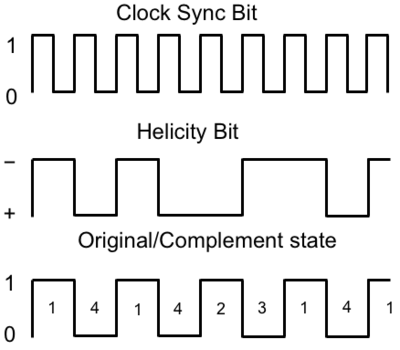
| − | The double spin asymmetry measurements performed in this thesis are performed by comparing scattering events that occur when the incident probe spin and nuclear target spin are parallel to scattering events that occur when the spins are anti-parallel. The helicity of the electron beam was flipped at a rate of 1 HZ. The helicity is prepared at the source such that helicity pairs are produced pseudo randomly. If the first electron bunch is pseudo randomly chosen to be positive (negative) then it is labeled as the original helicity state and denoted in software by a 2 (1). The next helicity state is prepared to be a complement to the first state and labeled in the software as either a 4, if the original helicity state was a 1 (negative), or 3 if the original helicity state was a 2 (positive. The helicity process is then repeated. Figure NES.1 illustrates the signals used to label helicity state. The clock pulse (SYNC) is used to indicate that a change in the pockel cell used to define the helicity state may have occurred. The helicity bit indicates the helicity state that was set. The original/complement pulse identifies if the state is an original or complement helicity state. All three bits are recorded in the raw data file for each event and then converted to the labels 1,2,3,4 during DST file production once the particles have been reconstructed. | + | The double spin asymmetry measurements performed in this thesis are performed by comparing scattering events that occur when the incident probe spin and nuclear target spin are parallel to scattering events that occur when the spins are anti-parallel. The helicity of the electron beam was flipped at a rate of 1 HZ. The helicity is prepared at the source such that helicity pairs are produced pseudo randomly. If the first electron bunch is pseudo randomly chosen to be positive (negative) then it is labeled as the original helicity state and denoted in software by a 2 (1). The next helicity state is prepared to be a complement to the first state and labeled in the software as either a 4, if the original helicity state was a 1 (negative), or 3 if the original helicity state was a 2 (positive). The helicity process is then repeated. Figure NES.1 illustrates the signals used to label helicity state. The clock pulse (SYNC) is used to indicate that a change in the pockel cell used to define the helicity state may have occurred. The helicity bit indicates the helicity state that was set. The original/complement pulse identifies if the state is an original or complement helicity state. All three bits are recorded in the raw data file for each event and then converted to the labels 1,2,3,4 during DST file production once the particles have been reconstructed. |
{| border="0" style="background:transparent;" align="center" | {| border="0" style="background:transparent;" align="center" | ||
| Line 1,594: | Line 1,594: | ||
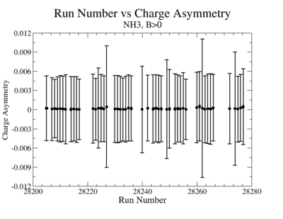
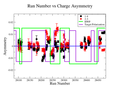
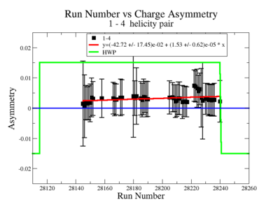
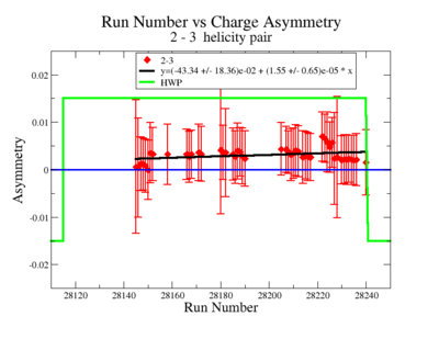
'''Figure NES. 2. Run Number vs the beam charge Asymmetry''' | '''Figure NES. 2. Run Number vs the beam charge Asymmetry''' | ||
|} | |} | ||
| + | |||
{| border="0" style="background:transparent;" align="center" | {| border="0" style="background:transparent;" align="center" | ||
| Line 1,603: | Line 1,604: | ||
|- | |- | ||
| | | | ||
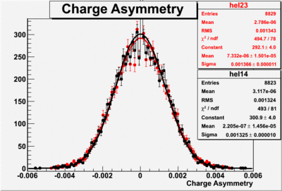
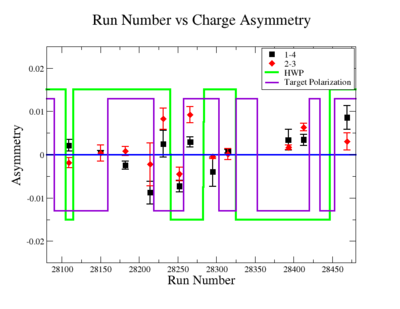
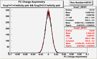
| − | '''Figure NES. 3. Beam charge asymmetry for 28101 | + | '''Figure NES. 3. Beam charge asymmetry for run #28101 using the gated faraday cup counts for two helicity pairs(1-4 and 2-3 helicity pairs).<math>A_{1-4}=(11.5 \pm 4.4) \times 10^{-5}</math> and <math>A_{2-3}=(-2.3 \pm 4.4) \times 10^{-5}</math>''' |
|} | |} | ||
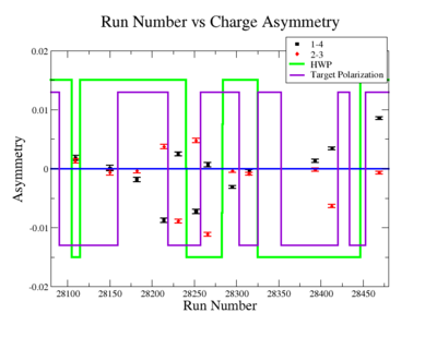
| + | |||
| + | [[File:RunNumber_vs_BeamChargeAsymmetryPulsePair14_19_03_2012.png|400px]][[File:RunNumber_vs_BeamChargeAsymmetryPulsePair23_19_03_2012.png|400px]] | ||
| + | |||
| + | {| border="1" |cellpadding="20" cellspacing="0 | ||
| + | |- | ||
| + | |Run Group || Half wave plane(HWP) || <math>A_{1-4}</math> || <math>A_{2-3}</math> | ||
| + | |- | ||
| + | | 28100 - 28105 || +1 || <math>(5.88 \pm 34.40) \times 10^{-4}</math> || <math>(4.03 \pm 34.36) \times 10^{-4}</math> | ||
| + | |- | ||
| + | | 28106 - 28115 || -1 ||<math> (7.53 \pm 22.30) \times 10^{-4}</math> ||<math> (8.28 \pm 22.30) \times 10^{-4}</math> | ||
| + | |- | ||
| + | | 28145 - 28240 || +1 || <math>(31.70 \pm 7.99) \times 10^{-4}</math> || <math>(30.40 \pm 7.99) \times 10^{-4}</math> | ||
| + | |- | ||
| + | | 28242 - 28284 || -1 ||<math> (49.6 \pm 10.8) \times 10^{-4}</math> ||<math> (47.9 \pm 10.8) \times 10^{-4}</math> | ||
| + | |- | ||
| + | | 28286 - 28324 || +1 ||<math> (36.3 \pm 11.6) \times 10^{-4}</math> ||<math> (37.0 \pm 11.5) \times 10^{-4}</math> | ||
| + | |- | ||
| + | | 28325 - 28447 || -1 ||<math> (21.1 \pm 13.4) \times 10^{-4}</math> || <math>(22.2 \pm 13.4) \times 10^{-4}</math> | ||
| + | |- | ||
| + | | 28449 - 28479 || +1 ||<math> (-11.6 \pm 16.5) \times 10^{-4}</math> || <math>(-21.6 \pm 16.5) \times 10^{-4}</math> | ||
| + | |} | ||
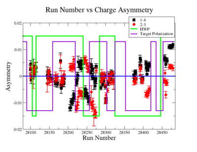
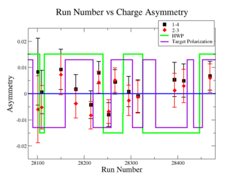
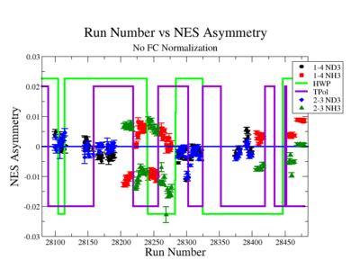
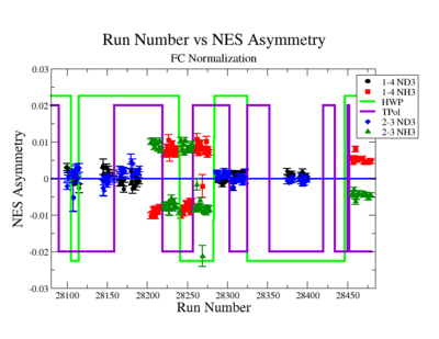
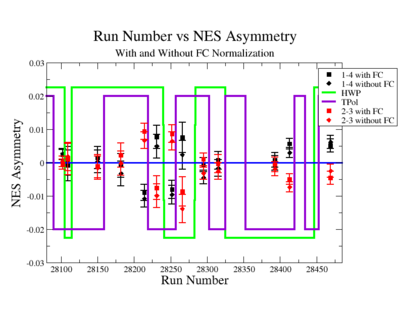
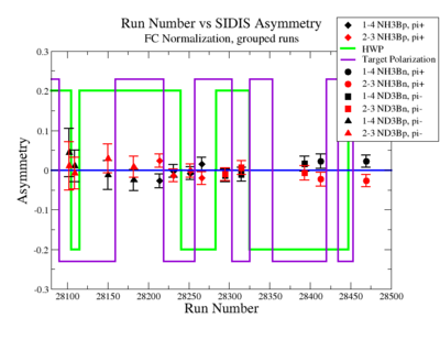
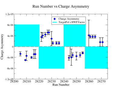
A measurement of the electron cross section helicity difference needs to account for the possible helicity dependence of the incident electron flux ( Charge Asymmetry). Fig. NES. 4 shows the reconstructed electron asymmetry before it is normalized by the gated Faraday Cup as a function of the run number for the 4.2 GeV data set. The reconstructed electron asymmetry can be defined following way: | A measurement of the electron cross section helicity difference needs to account for the possible helicity dependence of the incident electron flux ( Charge Asymmetry). Fig. NES. 4 shows the reconstructed electron asymmetry before it is normalized by the gated Faraday Cup as a function of the run number for the 4.2 GeV data set. The reconstructed electron asymmetry can be defined following way: | ||
| − | :::::<math>A_{NES}^{+-} = \frac{NES^{+} - NES^{-}}{NES^{+} + NES^{-}}</math> or <math>A_{NES}^{-+} = \frac{NES^{-} - NES^{+}}{NES^{-} + NES^{+}}</math> | + | :::::<math>A_{NES}^{+-} = \frac{NES^{+} - NES^{-}}{NES^{+} + NES^{-}} \equiv (2-3)</math> or <math>A_{NES}^{-+} = \frac{NES^{-} - NES^{+}}{NES^{-} + NES^{+}} \equiv (1-4)</math> |
where <math>NES^+</math>(<math>NES^-</math>) represents number of reconstructed electrons in the final state for the positive(negative) beam helicity. | where <math>NES^+</math>(<math>NES^-</math>) represents number of reconstructed electrons in the final state for the positive(negative) beam helicity. | ||
| Line 1,624: | Line 1,646: | ||
|} | |} | ||
| − | + | ||
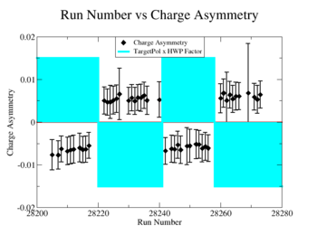
| + | Sysstematic effects on the asymmetry measurement may be investigated by separating the data into two groups based on which helicity state is set first. The first group(black data points) represents the electron asymmetry observed when the first (original) helicity state is negative and its complement state is positive(helicity state #1 - state #4). The second group(red data points) represents the asymmetry observed, when the first state is positive and the complement state is negative(helicity state #2 - #3). Both groups were divided into two subgroups based the target type used. The diamond points on the histogram represent the data for the NH3 target and the squares for the ND3 target. On the same histograms are presented the signs of the half wave plane(HWP) and the target polarization(TPol). The relative spin orientation can be changed by either inserting a half wave (HWP) or by populating a different target polarization state with a different RF frequency. One would expect the asymmetry to change sign if either the HWP is inserted or the target polarization is rotated 180 degrees. As one can see, the electron asymmetry sign ( sign(hel1-hel4) && sign(hel3-hel2) ) is opposite of the sign of (HWP<math>\times</math>Target_Polarization). The NES asymmetry has been calculated the following way before accounting for the Faraday cup: | ||
:::::::::<math>A_{NES} = \frac{NES^{hel1,hel2} - NES^{hel4,hel3}}{NES^{hel1,hel2} + NES^{hel4,hel3}}</math> | :::::::::<math>A_{NES} = \frac{NES^{hel1,hel2} - NES^{hel4,hel3}}{NES^{hel1,hel2} + NES^{hel4,hel3}}</math> | ||
| Line 1,703: | Line 1,726: | ||
| + | |||
| + | {| border="1" |cellpadding="20" cellspacing="0 | ||
| + | |- | ||
| + | | Target type, Beam Torus sign (B) || <math>A_{hel1-hel4}</math> || <math>A_{hel2-hel3}</math> || <math>A_{hel13-hel42}</math> | ||
| + | |- | ||
| + | | NH3, B>0, <math>\pi^+</math> || <math>(-139.84 \pm 81.52) \times 10^{-4}</math> | ||
| + | || <math>(143.15 \pm 81.78) \times 10^{-4}</math> ||<math> (-136.2 \pm 57.74) \times 10^{-4}</math> | ||
| + | |- | ||
| + | | NH3, B<0, <math>\pi^+</math> ||<math> (-223.76 \pm 117.10) \times 10^{-4}</math> | ||
| + | || <math>(247.65 \pm 116.59) \times 10^{-4}</math> || <math>(-237.69 \pm 82.65) \times 10^{-4}</math> | ||
| + | |- | ||
| + | | ND3, B>0, <math>\pi^-</math> || <math>(-6.37 \pm 188.73) \times 10^{-4}</math> | ||
| + | || <math>(-98.11 \pm 188.03) \times 10^{-4}</math> ||<math> (-9.21 \pm 127.22) \times 10^{-4}</math> | ||
| + | |- | ||
| + | | ND3, B<0, <math>\pi^-</math> || <math>(-63.73 \pm 105.14) \times 10^{-4}</math> | ||
| + | || <math>(-30.34 \pm 6085.54) \times 10^{-4}</math> ||<math> (-12.37 \pm 71.10) \times 10^{-4}</math> | ||
| + | |- | ||
| + | | NH3, B>0, <math>\pi^-</math> || <math>(-155.45 \pm 128.21) \times 10^{-4}</math> | ||
| + | || <math>(-72.55 \pm 128.92) \times 10^{-4}</math> ||<math>(-35.11 \pm 90.91) \times 10^{-4}</math> | ||
| + | |- | ||
| + | | NH3, B<0, <math>\pi^-</math> ||<math>(9.60 \pm 119.31) \times 10^{-4}</math>|| <math>(72.94 \pm 119.36) \times 10^{-4} | ||
| + | </math> || <math>(-32.39 \pm 84.38) \times 10^{-4}</math> | ||
| + | |- | ||
| + | | ND3, B>0, <math>\pi^+</math> || <math>(-76.59 \pm 126.60) \times 10^{-4}</math> | ||
| + | || <math>(110.28 \pm 126.13) \times 10^{-4}</math> ||<math> (-92.25 \pm 85.38) \times 10^{-4} </math> | ||
| + | |- | ||
| + | | ND3, B<0, <math>\pi^+</math> || <math>(-29.22 \pm 107.53) \times 10^{-4}</math> | ||
| + | || <math>(123.98 \pm 106.86) \times 10^{-4}</math> ||<math> (-92.25 \pm 85.38) \times 10^{-4}</math> | ||
| + | |} | ||
| + | |||
| + | |||
| + | {| border="1" |cellpadding="20" cellspacing="0 | ||
| + | |- | ||
| + | |Run Group || Target type, Beam Torus sign (B) || A_{1-4} || A_{2-3} | ||
| + | |- | ||
| + | | 28214 - || NH3, B>0 || <math>-0.02704757 \pm 0.01711263</math> || 0.02399480 \pm 0.01700174 | ||
| + | |- | ||
| + | | 28231 - || NH3, B>0 || <math>0.00069178 | ||
| + | \pm 0.01545227</math> || -0.01372286 | ||
| + | \pm 0.01559729 | ||
| + | |- | ||
| + | | 28252 - || NH3, B>0 || <math>-0.01229841 | ||
| + | \pm 0.01693271</math> || -0.00048034 \pm 0.01685103 | ||
| + | |- | ||
| + | | 28266 - || NH3, B>0 || <math>0.01589835 \pm 0.01590701</math> || -0.02002048 \pm 0.01610756 | ||
| + | |- | ||
| + | | 28413 - || NH3, B<0 || 0.02205009 \pm 0.01799869 || -0.02291024 \pm 0.01795956 | ||
| + | |- | ||
| + | | 28469 - || NH3, B<0 || 0.02270121 \pm 0.01543980 || -0.02662038 \pm 0.01532731 | ||
| + | |- | ||
| + | | 28102 - || ND3, B>0 || 0.04443768 \pm 0.06093347 || 0.01055158 \pm 0.06066387 | ||
| + | |- | ||
| + | | 28109 - || ND3, B>0 || 0.01068017 \pm 0.03953670 || -0.00764924 \pm 0.03970762 | ||
| + | |- | ||
| + | | 28150 - || ND3, B>0 || -0.01238850 \pm 0.03640693 || 0.02901657 \pm 0.03642766 | ||
| + | |- | ||
| + | | 28182 - || ND3, B>0 || -0.02497960 \pm 0.02660287 || 0.00797540 \pm 0.02634698 | ||
| + | |- | ||
| + | | 28295 - || ND3, B<0 || -0.01323095 \pm 0.01636848 || -0.01008145 \pm 0.01636433 | ||
| + | |- | ||
| + | | 28315 - || ND3, B<0 || -0.01026453 \pm 0.01768742 || 0.00621953 \pm 0.01758502 | ||
| + | |- | ||
| + | | 28393 - || ND3, B<0 || 0.01615151 \pm 0.01853525 || -0.00719786 \pm 0.01834110 | ||
| + | |} | ||
{| border="0" style="background:transparent;" align="center" | {| border="0" style="background:transparent;" align="center" | ||
| Line 1,714: | Line 1,801: | ||
'''Figure NES. 6. Run groups vs Semi inclusive asymmetry after FC Normalization.''' | '''Figure NES. 6. Run groups vs Semi inclusive asymmetry after FC Normalization.''' | ||
|} | |} | ||
| + | |||
| + | ===X and Z count distribution=== | ||
| + | |||
| + | |||
| + | {| border="1" |cellpadding="20" cellspacing="0 | ||
| + | |- | ||
| + | | SIDI Asymmetry || <math>X_B=0.3</math> || <math>X_B=0.4</math> | ||
| + | |- | ||
| + | |<math> A_{NH3}^{\pi^+,hel13-hel24}</math>||<math>(-150.08 \pm 65.96) \times 10^{-4}</math> || <math>(-217.20 \pm 69.06) \times 10^{-4}</math> | ||
| + | |- | ||
| + | |<math> A_{ND3}^{\pi^-,hel13-hel24}</math>||<math>(-39.04 \pm 81.44) \times 10^{-4}</math> || <math>(-91.90 \pm 96.14) \times 10^{-4}</math> | ||
| + | |- | ||
| + | |<math> A_{NH3}^{\pi^-,hel13-hel24}</math>||<math>(-100.81 \pm 83.49) \times 10^{-4}</math> || <math>(23.98 \pm 94.92) \times 10^{-4}</math> | ||
| + | |- | ||
| + | |<math> A_{ND3}^{\pi^+,hel13-hel24}</math>||<math>(-53.17 \pm 74.89) \times 10^{-4}</math> || <math>(-85.17 \pm 82.97) \times 10^{-4}</math> | ||
| + | |} | ||
| + | |||
| + | |||
| + | ====<math> A_{NH3}^{\pi^+,hel13-hel24}</math>==== | ||
| + | |||
| + | {| border="1" |cellpadding="20" cellspacing="0 | ||
| + | |- | ||
| + | | <math>z</math> || <math>X_B=0.3</math> || <math>X_B=0.4</math> | ||
| + | |- | ||
| + | | 0.3 ||<math>(-142.39 \pm 106.42) \times 10^{-4}</math> ||<math>( -131.49 \pm 116.96) \times 10^{-4}</math> | ||
| + | |- | ||
| + | | 0.5 || <math>(-101.14 \pm 128.36) \times 10^{-4}</math>||<math>(-207.76 \pm 129.37) \times 10^{-4}</math> | ||
| + | |- | ||
| + | | 0.7 ||<math>(-140.32 \pm 158.98) \times 10^{-4}</math>||<math>(-238.34 \pm 156.79) \times 10^{-4}</math> | ||
| + | |- | ||
| + | | 0.9 ||<math>(-355.44 \pm 200.23) \times 10^{-4}</math> ||<math>(-438.76 \pm 189.03) \times 10^{-4}</math> | ||
| + | |} | ||
| + | |||
| + | |||
| + | {| border="1" |cellpadding="20" cellspacing="0 | ||
| + | |- | ||
| + | | <math>z</math> || <math>X_B=0.3</math> || <math>X_B=0.4</math> | ||
| + | |- | ||
| + | | 0.45 ||<math>(-125.62 \pm 81.92) \times 10^{-4}</math> ||<math>( -165.81 \pm 86.76) \times 10^{-4}</math> | ||
| + | |- | ||
| + | | 0.7 ||<math>(-140.32 \pm 158.98) \times 10^{-4}</math>||<math>(-238.34 \pm 156.79) \times 10^{-4}</math> | ||
| + | |- | ||
| + | | 0.9 ||<math>(-355.44 \pm 200.23) \times 10^{-4}</math> ||<math>(-438.76 \pm 189.03) \times 10^{-4}</math> | ||
| + | |} | ||
| + | |||
| + | ====<math> A_{ND3}^{\pi^-,hel13-hel24}</math>==== | ||
| + | |||
| + | {| border="1" |cellpadding="20" cellspacing="0 | ||
| + | |- | ||
| + | | <math>z</math> || <math>X_B=0.3</math> || <math>X_B=0.4</math> | ||
| + | |- | ||
| + | | 0.3 ||<math>(9.18 \pm 120.73) \times 10^{-4}</math> ||<math>( -46.32 \pm 147.45) \times 10^{-4}</math> | ||
| + | |- | ||
| + | | 0.5 || <math>(-66.91 \pm 161.28) \times 10^{-4}</math>||<math>(-78.88 \pm 182.05) \times 10^{-4}</math> | ||
| + | |- | ||
| + | | 0.7 ||<math>(-96.54 \pm 232.06) \times 10^{-4}</math>||<math>(-236.67 \pm 257.03) \times 10^{-4}</math> | ||
| + | |- | ||
| + | | 0.9 ||<math>(-147.74 \pm 297.50) \times 10^{-4}</math> ||<math>(-78.69 \pm 320.29) \times 10^{-4}</math> | ||
| + | |} | ||
| + | |||
| + | |||
| + | <math>\Delta R_{np}^{\pi^+ + \pi^-} = \frac{\Delta \sigma_p^{\pi^+ + \pi^-} - \Delta \sigma_{n}^{\pi^+ + \pi^-}}{\sigma_p^{\pi^+ + \pi^-} - \sigma_{n}^{\pi^+ + \pi^-}}=</math> | ||
| + | |||
| + | <math>=\frac{\Delta \sigma_p^{\pi^+ + \pi^-}}{\sigma_p^{\pi^+ + \pi^-} - \sigma_{n}^{\pi^+ + \pi^-}} - \frac{\Delta \sigma_{n}^{\pi^+ + \pi^-}}{\sigma_p^{\pi^+ + \pi^-} - \sigma_{n}^{\pi^+ + \pi^-}}=</math> | ||
| + | |||
| + | <math> = \frac{(\sigma_p^{\pi^+,hel13} - \sigma_p^{\pi^+,hel24}) + (\sigma_p^{\pi^-,hel13} - \sigma_p^{\pi^-,hel24})}{\sigma_p^{\pi^+ + \pi^-} - \sigma_{n}^{\pi^+ + \pi^-}} - \frac{(\sigma_n^{\pi^+,hel13} - \sigma_n^{\pi^+,hel24}) + (\sigma_n^{\pi^-,hel13} - \sigma_n^{\pi^-,hel24})}{\sigma_p^{\pi^+ + \pi^-} - \sigma_{n}^{\pi^+ + \pi^-}} = </math> | ||
| + | |||
| + | |||
| + | |||
| + | <math>=\frac{(\Delta u +\Delta \bar{u}) - (\Delta d + \Delta \bar{d})}{(u+\bar{u}) - (d+\bar{d})}(x,Q^2)=</math> | ||
| + | |||
| + | |||
| + | |||
| + | <math>= \frac{g_1^p - g_1^n}{F_1^p - F_1^n}(x,Q^2)</math> | ||
| + | |||
| + | |||
| + | "If each observable (<math>x_i</math>) is accompanied by an estimate of the uncertainty in that observable (<math>\sigma_i</math>) then the weighted mean is defined as | ||
| + | |||
| + | :<math>\bar{x} = \frac{ \sum_{i=1}^{i=n} \frac{x_i}{\sigma_i^2}}{\sum_{i=1}^{i=n} \frac{1}{\sigma_i^2}}</math>" | ||
| + | |||
| + | "The variance of the distribution is defined as | ||
| + | |||
| + | :<math>\frac{1}{\sigma^2} = \sum_{i=1}^{i=n} \frac{1}{\sigma_i^2}</math> = weighted variance" | ||
| + | [[TF_ErrorAna_PropOfErr]] | ||
| + | |||
| + | {| border="1" style="text-align: center;" align="center" | ||
| + | |- | ||
| + | | <math>z</math> || <math>X_B=0.3</math> || <math>X_B=0.4</math> | ||
| + | |- | ||
| + | | 0.3 ||<math>(1453.94 | ||
| + | \pm 236.39) \times 10^{-4}</math> ||<math>(-104.24 \pm 277.69) \times 10^{-4}</math> | ||
| + | |- | ||
| + | | 0.5 ||<math>(550.18 \pm 298.65) \times 10^{-4}</math>||<math>(149.78 \pm 320.13) \times 10^{-4}</math> | ||
| + | |- | ||
| + | | 0.7 ||<math>(-650.12 | ||
| + | \pm 407.30) \times 10^{-4}</math> ||<math>(79.69 \pm 430.29) \times 10^{-4}</math> | ||
| + | |- | ||
| + | | 0.9 ||<math>(2285.22 \pm 525.13) \times 10^{-4}</math>||<math>(5.59 \pm 545.08) \times 10^{-4}</math> | ||
| + | |} | ||
| + | {| border="0" style="background:transparent;" align="center" | ||
| + | |- | ||
| + | |'''Table 4.5.''' Experimental Results of The Fragmentation Function <math>\Delta R_{np}^{\pi^+ + \pi^-} </math> vs <math>z</math> and <math>X_B</math> for four values of <math>z</math>. | ||
| + | |}<br><br> | ||
| + | |||
| + | {| border="1" style="text-align: center;" align="center" | ||
| + | |- | ||
| + | | <math>z</math> || <math>X_B=0.3</math> || <math>X_B=0.4</math> | ||
| + | |- | ||
| + | | 0.45 ||<math>(582.79 | ||
| + | \pm 186.97) \times 10^{-4}</math> ||<math>( 55.32 \pm 214.92) \times 10^{-4}</math> | ||
| + | |- | ||
| + | | 0.85 ||<math>(504.20 \pm 321.74) \times 10^{-4}</math>||<math>(57.35 \pm 337.48) \times 10^{-4}</math> | ||
| + | |} | ||
| + | {| border="0" style="background:transparent;" align="center" | ||
| + | |- | ||
| + | |'''Table 4.6.''' Experimental Results of The Fragmentation Function <math>\Delta R_{np}^{\pi^+ + \pi^-} </math> vs <math>z</math> and <math>X_B</math>(Combined <math>z</math>). | ||
| + | |}<br> | ||
| + | |||
| + | |||
| + | {| border="1" style="text-align: center;" align="center" | ||
| + | |- | ||
| + | | <math>Q^{2}</math> || <math>W^{2}</math> || <math>X_{b}</math> || <math>\Delta R_{deuteron,p}^{\pi^+ + \pi^-} </math> || <math>\Delta R_{np}^{\pi^+ + \pi^-} </math> | ||
| + | |- | ||
| + | | 0.8 || 2.4 || 0.344712 || 0.089457 || 1.215956 | ||
| + | |- | ||
| + | | 0.8 || 2.56 || 0.322805 || 0.087636 || 1.144319 | ||
| + | |- | ||
| + | | 0.8 || 2.72 || 0.302941 || 0.087324 || 1.142601 | ||
| + | |- | ||
| + | | 0.8 || 2.89 || 0.284872 || 0.080418 || 1.081259 | ||
| + | |- | ||
| + | | 0.8 || 3.06 || 0.268386 || 0.046144 || 0.971948 | ||
| + | |- | ||
| + | | 0.8 || 3.24 || 0.253303 || -0.001413 || 0.904000 | ||
| + | |- | ||
| + | | 0.8 || 3.42 || 0.239465 || -0.039615 || 0.888457 | ||
| + | |- | ||
| + | | 0.85 || 2.4 || 0.358532 || 0.095124 || 1.179011 | ||
| + | |- | ||
| + | | 0.85 || 2.56 || 0.336197 || 0.092376 || 1.118478 | ||
| + | |- | ||
| + | | 0.85 || 2.72 || 0.315894 || 0.091414 || 1.126200 | ||
| + | |- | ||
| + | | 0.85 || 2.89 || 0.297382 || 0.083684 || 1.073062 | ||
| + | |- | ||
| + | | 0.85 || 3.06 || 0.280456 || 0.047397 || 0.965145 | ||
| + | |- | ||
| + | | 0.85 || 3.24 || 0.264940 || 0.000751 || 0.897095 | ||
| + | |- | ||
| + | | 0.85 || 3.42 || 0.250680 || -0.037185 || 0.879470 | ||
| + | |- | ||
| + | | 0.9 || 2.4 || 0.371781 || 0.101758 || 1.124929 | ||
| + | |- | ||
| + | | 0.9 || 2.56 || 0.349070 || 0.097293 || 1.077209 | ||
| + | |- | ||
| + | | 0.9 || 2.72 || 0.328374 || 0.095640 || 1.097502 | ||
| + | |- | ||
| + | | 0.9 || 2.89 || 0.309461 || 0.087175 || 1.064119 | ||
| + | |- | ||
| + | | 0.9 || 3.06 || 0.292134 || 0.050127 || 0.968564 | ||
| + | |- | ||
| + | | 0.9 || 3.24 || 0.276219 || 0.003136 || 0.902680 | ||
| + | |- | ||
| + | | 0.9 || 3.42 || 0.261569 || -0.034673 || 0.882556 | ||
| + | |- | ||
| + | | 0.95 || 2.4 || 0.384494 || 0.107726 || 1.079087 | ||
| + | |- | ||
| + | | 0.95 || 2.56 || 0.361453 || 0.102269 || 1.040995 | ||
| + | |- | ||
| + | | 0.95 || 2.72 || 0.340407 || 0.099848 || 1.072015 | ||
| + | |- | ||
| + | | 0.95 || 2.89 || 0.321133 || 0.090544 || 1.055804 | ||
| + | |- | ||
| + | | 0.95 || 3.06 || 0.303439 || 0.052833 || 0.971023 | ||
| + | |- | ||
| + | | 0.95 || 3.24 || 0.287158 || 0.005393 || 0.907107 | ||
| + | |- | ||
| + | | 0.95 || 3.42 || 0.272146 || -0.032200 || 0.884625 | ||
| + | |- | ||
| + | | 1 || 2.4 || 0.396703 || 0.113466 || 1.036707 | ||
| + | |- | ||
| + | | 1 || 2.56 || 0.373374 || 0.106727 || 1.007923 | ||
| + | |- | ||
| + | | 1 || 2.72 || 0.352016 || 0.103726 || 1.047463 | ||
| + | |- | ||
| + | | 1 || 2.89 || 0.332416 || 0.093605 || 1.045933 | ||
| + | |- | ||
| + | | 1 || 3.06 || 0.314388 || 0.055305 || 0.970792 | ||
| + | |- | ||
| + | | 1 || 3.24 || 0.297772 || 0.007453 || 0.909048 | ||
| + | |- | ||
| + | | 1 || 3.42 || 0.282424 || -0.029966 || 0.884723 | ||
| + | |- | ||
| + | | 1.05 || 2.4 || 0.408437 || 0.118939 || 0.992592 | ||
| + | |- | ||
| + | | 1.05 || 2.56 || 0.384858 || 0.111105 || 0.971331 | ||
| + | |- | ||
| + | | 1.05 || 2.72 || 0.363224 || 0.107103 || 1.019267 | ||
| + | |- | ||
| + | | 1.05 || 2.89 || 0.343330 || 0.095852 || 1.029986 | ||
| + | |- | ||
| + | | 1.05 || 3.06 || 0.324999 || 0.057266 || 0.964081 | ||
| + | |- | ||
| + | | 1.05 || 3.24 || 0.308073 || 0.009820 || 0.906637 | ||
| + | |- | ||
| + | | 1.05 || 3.42 || 0.292416 || -0.027198 || 0.883994 | ||
| + | |- | ||
| + | | 1.1 || 2.4 || 0.419723 || 0.125251 || 0.947155 | ||
| + | |- | ||
| + | | 1.1 || 2.56 || 0.395929 || 0.115416 || 0.938049 | ||
| + | |- | ||
| + | | 1.1 || 2.72 || 0.374051 || 0.110297 || 0.993433 | ||
| + | |- | ||
| + | | 1.1 || 2.89 || 0.353894 || 0.098076 || 1.014245 | ||
| + | |- | ||
| + | | 1.1 || 3.06 || 0.335286 || 0.059359 || 0.956429 | ||
| + | |- | ||
| + | | 1.1 || 3.24 || 0.318077 || 0.012982 || 0.905373 | ||
| + | |- | ||
| + | | 1.1 || 3.42 || 0.302133 || -0.024350 || 0.882958 | ||
| + | |- | ||
| + | | 1.15 || 2.4 || 0.430586 || 0.130979 || 0.910430 | ||
| + | |- | ||
| + | | 1.15 || 2.56 || 0.406608 || 0.119423 || 0.907506 | ||
| + | |- | ||
| + | | 1.15 || 2.72 || 0.384515 || 0.113163 || 0.969323 | ||
| + | |- | ||
| + | | 1.15 || 2.89 || 0.364122 || 0.100019 || 0.998793 | ||
| + | |- | ||
| + | | 1.15 || 3.06 || 0.345265 || 0.061046 || 0.948539 | ||
| + | |- | ||
| + | | 1.15 || 3.24 || 0.327796 || 0.015164 || 0.901680 | ||
| + | |- | ||
| + | | 1.15 || 3.42 || 0.311587 || -0.021709 || 0.880861 | ||
| + | |- | ||
| + | | 1.2 || 2.4 || 0.441050 || 0.136174 || 0.877989 | ||
| + | |- | ||
| + | | 1.2 || 2.56 || 0.416916 || 0.123376 || 0.879867 | ||
| + | |- | ||
| + | | 1.2 || 2.72 || 0.394636 || 0.116022 || 0.947092 | ||
| + | |- | ||
| + | | 1.2 || 2.89 || 0.374032 || 0.101867 || 0.984262 | ||
| + | |- | ||
| + | | 1.2 || 3.06 || 0.354948 || 0.062766 || 0.940538 | ||
| + | |- | ||
| + | | 1.2 || 3.24 || 0.337242 || 0.017174 || 0.897860 | ||
| + | |- | ||
| + | | 1.2 || 3.42 || 0.320789 || -0.019216 || 0.878344 | ||
| + | |- | ||
| + | | 1.25 || 2.4 || 0.451137 || 0.141522 || 0.851328 | ||
| + | |- | ||
| + | | 1.25 || 2.56 || 0.426872 || 0.127836 || 0.854448 | ||
| + | |- | ||
| + | | 1.25 || 2.72 || 0.404429 || 0.119066 || 0.924399 | ||
| + | |- | ||
| + | | 1.25 || 2.89 || 0.383638 || 0.104151 || 0.966286 | ||
| + | |- | ||
| + | | 1.25 || 3.06 || 0.364349 || 0.064626 || 0.929040 | ||
| + | |- | ||
| + | | 1.25 || 3.24 || 0.346426 || 0.019518 || 0.890588 | ||
| + | |- | ||
| + | | 1.25 || 3.42 || 0.329748 || -0.016436 || 0.873707 | ||
| + | |- | ||
| + | | 1.3 || 2.4 || 0.460866 || 0.146979 || 0.827067 | ||
| + | |- | ||
| + | | 1.3 || 2.56 || 0.436494 || 0.131843 || 0.832123 | ||
| + | |- | ||
| + | | 1.3 || 2.72 || 0.413910 || 0.122206 || 0.903273 | ||
| + | |- | ||
| + | | 1.3 || 2.89 || 0.392954 || 0.106218 || 0.949548 | ||
| + | |- | ||
| + | | 1.3 || 3.06 || 0.373480 || 0.066537 || 0.917721 | ||
| + | |- | ||
| + | | 1.3 || 3.24 || 0.355358 || 0.021675 || 0.883594 | ||
| + | |- | ||
| + | | 1.3 || 3.42 || 0.338473 || -0.013711 || 0.868901 | ||
| + | |- | ||
| + | | 1.35 || 2.4 || 0.470256 || 0.151920 || 0.806259 | ||
| + | |- | ||
| + | | 1.35 || 2.56 || 0.445798 || 0.135925 || 0.812231 | ||
| + | |- | ||
| + | | 1.35 || 2.72 || 0.423094 || 0.125351 || 0.884403 | ||
| + | |- | ||
| + | | 1.35 || 2.89 || 0.401992 || 0.108521 || 0.933955 | ||
| + | |- | ||
| + | | 1.35 || 3.06 || 0.382352 || 0.068511 || 0.907321 | ||
| + | |- | ||
| + | | 1.35 || 3.24 || 0.364050 || 0.023938 || 0.877039 | ||
| + | |- | ||
| + | | 1.35 || 3.42 || 0.346974 || -0.011047 || 0.864389 | ||
| + | |}<br> | ||
| + | {| border="0" style="background:transparent;" align="center" | ||
| + | |- | ||
| + | |'''Table 4.7.''' <math> \frac{g_1^p - g_1^n}{F_1^p - F_1^n}(x,Q^2)</math>. | ||
| + | |}<br> | ||
| + | |||
| + | |||
| + | {| border="1" style="text-align: center;" align="center" | ||
| + | |- | ||
| + | | <math>n_{C,MT,\pi^{+} \pi^{-}}</math> || <math>x_{B}=0.3</math> || <math>x_{B}=0.4</math> | ||
| + | |- | ||
| + | | <math>n_{C,\pi^{+}}</math>, <math>z=0.45</math> || 0.006584 || 0.004943 | ||
| + | |- | ||
| + | | <math>n_{C,\pi^{-}}</math>, <math>z=0.45</math> || 0.006382 || 0.004355 | ||
| + | |- | ||
| + | | <math>n_{MT,\pi^{+}}</math>, <math>z=0.45</math> || 0.005769 || 0.004544 | ||
| + | |- | ||
| + | | <math>n_{MT,\pi^{-}}</math>, <math>z=0.45</math> || 0.005856 || 0.004021 | ||
| + | |- | ||
| + | | <math>n_{C,\pi^{+}}</math>, <math>z=0.85</math> || 0.002893 || 0.002574 | ||
| + | |- | ||
| + | | <math>n_{C,\pi^{-}}</math>, <math>z=0.85</math> || 0.001664 || 0.001361 | ||
| + | |- | ||
| + | | <math>n_{MT,\pi^{+}}</math>, <math>z=0.85</math> || 0.002673 || 0.002399 | ||
| + | |- | ||
| + | | <math>n_{MT,\pi^{-}}</math>, <math>z=0.85</math> || 0.001565 || 0.001307 | ||
| + | |}<br> | ||
| + | |||
| + | {| border="1" style="text-align: center;" align="center" | ||
| + | |- | ||
| + | | <math>n_{NH3,ND,\pi^{+} \pi^{-}}</math> || <math>x_{B}=0.3</math> || <math>x_{B}=0.4</math> | ||
| + | |- | ||
| + | | <math>n_{NH3,\pi^{+}}</math>, <math>z=0.45</math> || 0.00611464 | ||
| + | || 0.00545206 | ||
| + | |- | ||
| + | | <math>n_{NH3,\pi^{-}}</math>, <math>z=0.45</math> || 0.00428864 | ||
| + | || 0.00330646 | ||
| + | |- | ||
| + | | <math>n_{ND3,\pi^{+}}</math>, <math>z=0.45</math> || 0.00552027 | ||
| + | || 0.00392858 | ||
| + | |- | ||
| + | | <math>n_{ND3,\pi^{-}}</math>, <math>z=0.45</math> || 0.00552027 | ||
| + | || 0.00392858 | ||
| + | |- | ||
| + | | <math>n_{NH3,\pi^{+}}</math>, <math>z=0.85</math> || 0.00265003 | ||
| + | || 0.00282080 | ||
| + | |- | ||
| + | | <math>n_{NH3,\pi^{-}}</math>, <math>z=0.85</math> || 0.00097612 | ||
| + | || 0.00090184 | ||
| + | |- | ||
| + | | <math>n_{ND3,\pi^{+}}</math>, <math>z=0.85</math> || 0.00264221 | ||
| + | || 0.00243020 | ||
| + | |- | ||
| + | | <math>n_{ND3,\pi^{-}}</math>, <math>z=0.85</math> ||0.00154130 | ||
| + | || 0.00128547 | ||
| + | |}<br> | ||
| + | |||
| + | {| border="1" style="text-align: center;" align="center" | ||
| + | |- | ||
| + | |<math>x_{B}=0.3</math> || <math>x_{B}=0.4</math> | ||
| + | |- | ||
| + | | <math>0.969 \pm 0.095</math> || <math>0.947 \pm 0.08</math> | ||
| + | |}<br> | ||
| + | {| border="0" style="background:transparent;" align="center" | ||
| + | |- | ||
| + | |'''Table 4.7.''' Average <math> \Delta R_{np}^{\pi^+ + \pi^-} = \frac{g_1^p - g_1^n}{F_1^p - F_1^n}(x,Q^2)</math>. | ||
| + | |}<br> | ||
| + | |||
| + | |||
| + | {| border="1" style="text-align: center;" align="center" | ||
| + | |- | ||
| + | | <math>z</math> || <math>X_B=0.3</math> || <math>X_B=0.4</math> | ||
| + | |- | ||
| + | | 0.45 ||<math>-0.297 \pm 0.071</math> ||<math> -0.379 \pm 0.071</math> | ||
| + | |- | ||
| + | | 0.7 ||<math>-0.120 \pm 0.072</math>||<math>-0.122 \pm 0.072</math> | ||
| + | |}<br> | ||
| + | |||
| + | |||
| + | [http://wiki.iac.isu.edu/index.php/User_talk:Didbtama Go Back] | ||
Latest revision as of 05:07, 8 December 2012
TD_Ddoverd_2008
TD_Ddoverd_2009
TD_Ddoverd_2010
The goal
Fragmentation Function test
A complete test of independent fragmentation can be performed with polarized proton and neutron targets. The ratio of the difference of polarized to unpolarized cross sections for proton and neutron targets can be written in terms of the structure functions:
Delta d over d
1/24/2011
1.) Find energy range with substantial ND3, pi- events when B <0.
Ratio plot for Q^2 and X_{BJ}
once you find the Q^2 and X_BJ range holding a reasonable amount of data.
2.) Inclusive electron scattering ratio of
| Inclusiveelectrons -vs- Q-squared | Inclusive Missing Mass (W) for 1.0 Q^2 <1.2 |
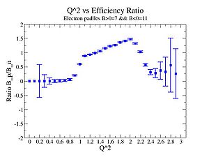
| [[|300px|thumb|The ratio of inclusive electrons detected in scintillator paddle #7 when Btorus >0 (B_p)to inclusive electrons detected by paddle 11 when B<0(B_n) NH3 Target]] | [[|300px|thumb|The inclusive missing mass W for each torus setting. Dashed line is B>0 and solid line is B<0]] |
| [[|300px|thumb|The ratio of inclusive electrons detected in scintillator paddle #7 when Btorus >0 (B_p)to inclusive electrons detected by paddle 11 when B<0(B_n)]]ND3 Target | [[|300px|thumb|The inclusive missing mass W for each torus setting. Dashed line is B>0 and solid line is B<0]] |
| [[|300px|thumb|The ratio of inclusive electrons detected in scintillator paddle #7 when Btorus >0 (B_p)to inclusive electrons detected by paddle 11 when B<0(B_n)]] Both Targets | 300px|thumb|The inclusive missing mass W for each torus setting. Dashed line is B>0 and solid line is B<0 |
3.) Semi Inclusive pion production ratios -vs- Q^2, Only electron cuts
/cache/mss/clas/eg1b/production/pass1/v4/4p2out/misc/dst/dst2828*
ND3 4.2-
28287 28288 28289 28290 28291 28292 28293 28294 28295 28296 28298 28299 28300 28301 28302 28306 28307 28309 28311 28312 28313 28314 28315 28316 28317 28319 28320 28321 28322 28323 28335 28336 28337 28338 28339 28340 28341 28351 28352 28367 28368 28369 28370 28371 28372 28373 28374 28375 28376 28377 28378 28379 28380 28381 28385 28386 28389 28390 28391 28392 28393 28394 28396 28397 28398 28399 28400 28401
ND3 4.2+
28074 28075 28076 28077 28078 28079 28081 28082 28083 28086 28087 28088 28089 28093 28094 28095 28096 28097 28098 28099 28100 28101 28102 28106 28107 28108 28109 28110 28111 28112 28113 28115 28145 28146 28147 28148 28149 28152 28154 28158 28166 28167 28168 28171 28172 28180 28181 28182 28185 28186 28187 28188 28189 28190
NH3 4.2-
28407 28408 28409 28410 28411 28412 28413 28414 28415 28416 28417 28422 28423 28424 28425 28426 28427 28428 28429 28432 28433 28438 28439 28443 28445 28446 28447 28448 28449 28450 28456 28457 28458 28460 28461 28462 28463 28464 28467 28469 28471 28472 28473 28476 28478 28479
NH3 4.2+
28205 28207 28208 28209 28210 28211 28212 28214 28215 28216 28217 28222 28223 28224 28225 28226 28227 28230 28231 28232 28233 28234 28235 28236 28240 28242 28244 28245 28246 28247 28249 28250 28252 28253 28254 28255 28256 28260 28261 28262 28263 28264 28265 28266 28272 28274 28275 28276 28277
File locations:
http://www.jlab.org/Hall-B/secure/eg1/EG2000/nevzat/UPGRADE_DST/
/cache/mss/clas/eg1b/production/pass1/v4/4p2out/misc/dst/dst2828*
/cache/mss/home/nguler/dst
Rates before and after requiring pions
all the cuts are applied, except NPHE>2.5 cut.
4.2 GeV, ND3 target, 98 files, B<0
4.2 GeV, ND3 target, 32 files, B>0
The ratio for ND3 4.2 GeV data
Electron paddle selection
Inclusive
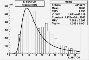 |
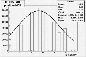
|
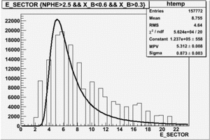
| Electron Paddle Number(Inclusive, B<0, 4.2 GeV Beam, ND3 Target) | Electron Paddle Number(Inclusive, B>0, 4.2 GeV Beam, ND3 Target) |
Semi-Inclusive
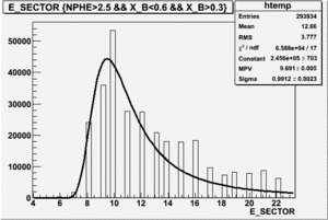 |
|
| Electron Paddle Number(Semi-Inclusive, B<0, 4.2 GeV Beam, ND3 Target) | Electron Paddle Number(Semi-Inclusive, B>0, 4.2 GeV Beam, ND3 Target) |
B>0, ND3 Electron paddle number=5
B<0, ND3 Electron paddle number=10
The Ratio
| X_B | without pions | with pions |
| 0.3 | ||
| 0.35 | ||
| 0.4 | ||
| 0.45 | ||
| 0.5 | ||
| 0.55 |
The ratio for NH3 4.2 GeV data
Electron paddle selection
Inclusive
 |
|
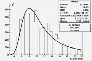
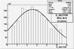
| Electron Paddle Number(Inclusive, B<0, NH3 target, 4.2 GeV Beam) | Electron Paddle Number(Inclusive, B>0, NH3 target, 4.2 GeV Beam) |
Semi-Inclusive
 |
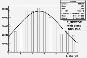
|
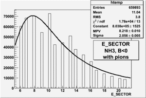
| Electron Paddle Number(Semi-Inclusive, B<0, NH3 target, 4.2 GeV Beam) | Electron Paddle Number(Semi-Inclusive, B>0, NH3 target, 4.2 GeV Beam) |
B>0, NH3 Electron paddle number=5
B<0, NH3 Electron paddle number=10
The Ratio
| X_B | without pions | with pions |
| 0.3 | ||
| 0.35 | ||
| 0.4 | ||
| 0.45 | ||
| 0.5 | ||
| 0.55 |
1/31/11
Electron paddle number for B>0 is 5 and for B<0 - 10. The cut was applied on :
Inclusive
1.) Overlap electron kinematic (, W, Momentum) for B>0 and B<0 and ND3 and NH3.
(NH3,B>0), (NH3,B<0), (ND3,B>0) && (ND3,B<0)
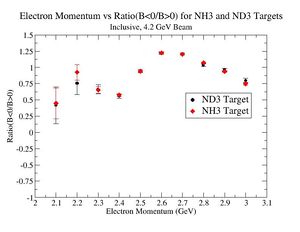
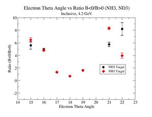
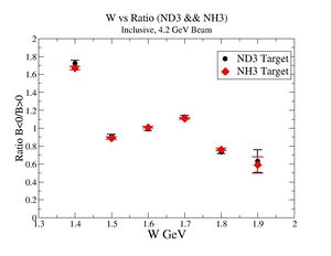
2.) Now plot ratio (B< 0/B>0) electron kinematic (, W, Momentum) for ND3 and NH3. ( I expect 2 curves in one plot)
,
 |
 |
|
| Electron Momentum(, ) | Electron Angle(, ) | W mass(, ) |
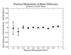
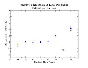
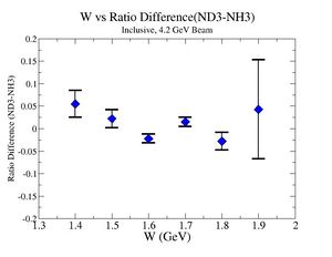
2.) Target ratio (B< 0/B>0) Difference electron kinematic (, W, Momentum) (Ration for ND3 target - Ratio for NH3 target). ( I expect 1 curves in one plot)
 |
 |
|
| Electron Momentum () | Theta Angle() | W mass() |
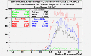
Semi-Inclusive
(NH3,B>0), (NH3,B<0), (ND3,B>0) && (ND3,B<0)
 |
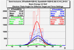 |
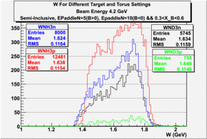
|
| Electron Momentum((NH3,B>0), (NH3,B<0), (ND3,B>0) && (ND3,B<0)) | Electron Angle((NH3,B>0), (NH3,B<0), (ND3,B>0) && (ND3,B<0)) | W mass((NH3,B>0), (NH3,B<0), (ND3,B>0) && (ND3,B<0)) |
2
2/7/11
1.) Now look a specific electron kinematic which appear to have unity ratio. P=2.5 GeV, \theta =18 degrees
| W | NH3,B<0 | NH3,B>0 | ND3,B<0 | ND3,B>0 | NH3,B>0 - NH3,B<0 | NH3,B>0 - NH3,B<0 |
| 1.72 | 1.7 | -9.7 | ||||
| 1.74 | 3 | 5.1 | -3.2 | |||
| 1.76 | 5.0 | -43.6 | ||||
| 1.78 | 4.2 | -33.1 | ||||
| 1.8 | 0.8 | -5.2 |
2.) Semi-Inclusive using above electrons
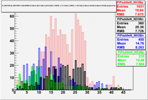 |
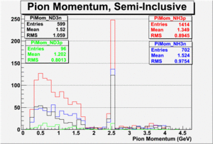
|
| Paddle Number | Pion Momentum |
3.) Semi-Inclusive using above electrons and choosing a single paddle from 2.)
| Pi+/Pi- hitting paddle # | Pi+/Pi- hitting paddle # |
2/14/11
1.) Get all files
2.) Do semi-inclusive paddle number for pions again
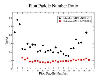
3.) Paddle Number ratio (with more files in order to double check, the same cuts on electrons)
2/23/11
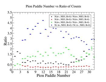
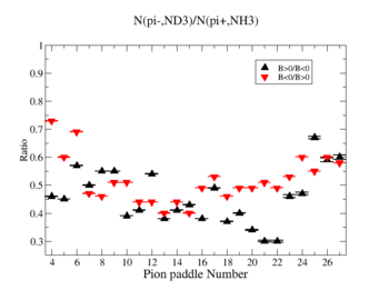
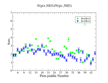
1.) Plot pi^-/pi^+ -vs paddle #
2.) Paddle 7 has ratio 0f 0.9. Plot W, Q^2 and M_{\pi}
W
Q^2
3.) Paddle 25 has ratio 0f 0.3. Plot W, Q^2, M (our goal is to determine if the detector has same efficiency for detector same reaction when the Torus filed is flipped)
W
Q^2
3/04/11
Table. 1 Pion Paddle Number ratio
- 1.) ND3Bn/NH3Bp
| Pion Paddle Number | Number of Events ND3Bn | Number of Events NH3Bp | Ratio(ND3Bn/NH3Bp) error |
| 3.89 | 81 | 69 | 0.4 0.000896 |
| 4.89 | 84 | 87 | 0.33 0.000595 |
| 5.89 | 84 | 76 | 0.38 0.000757 |
| 6.89 | 75 | 98 | 0.26 0.000488 |
| 7.89 | 91 | 123 | 0.25 0.000348 |
| 8.89 | 115 | 141 | 0.28 0.000283 |
| 9.89 | 207 | 254 | 0.28 0.000117 |
| 10.89 | 212 | 300 | 0.24 0.000092 |
| 11.89 | 284 | 413 | 0.24 0.000057 |
| 12.89 | 322 | 501 | 0.22 0.000043 |
| 13.89 | 359 | 521 | 0.24 0.000040 |
| 14.89 | 365 | 565 | 0.22 0.000036 |
| 15.89 | 415 | 523 | 0.27 0.000040 |
| 16.89 | 444 | 526 | 0.29 0.000039 |
| 17.89 | 405 | 555 | 0.25 0.000036 |
| 18.89 | 414 | 528 | 0.27 0.000039 |
| 19.89 | 387 | 502 | 0.27 0.000042 |
| 20.89 | 408 | 505 | 0.28 0.000042 |
| 21.89 | 352 | 457 | 0.27 0.000048 |
| 22.89 | 298 | 358 | 0.29 0.000070 |
| 23.89 | 522 | 547 | 0.33 0.000038 |
| 24.89 | 530 | 608 | 0.3 0.000032 |
| 25.89 | 571 | 590 | 0.33 0.000034 |
| 26.89 | 523 | 564 | 0.32 0.000036 |
| 27.89 | 422 | 440 | 0.33 0.000052 |
| 28.89 | 368 | 342 | 0.37 0.000079 |
| 29.89 | 101 | 108 | 0.32 0.000427 |
- 2.) ND3Bp/NH3Bn
| Pion Paddle Number | Number of Events ND3Bp | Number of Events NH3Bn | Ratio(ND3Bp/NH3Bn) error |
| 0.91 | 45 | 89 | 1.29 0.004556 |
| 1.91 | 86 | 127 | 1.73 0.002488 |
| 2.91 | 82 | 133 | 1.58 0.002361 |
| 3.91 | 91 | 330 | 0.71 0.000822 |
| 4.91 | 94 | 348 | 0.69 0.000766 |
| 5.91 | 125 | 360 | 0.89 0.000649 |
| 6.91 | 120 | 399 | 0.77 0.000594 |
| 7.91 | 148 | 443 | 0.86 0.000484 |
| 8.91 | 128 | 387 | 0.85 0.000595 |
| 9.91 | 121 | 510 | 0.61 0.000459 |
| 10.91 | 104 | 417 | 0.64 0.000607 |
| 11.91 | 145 | 449 | 0.83 0.000481 |
| 12.91 | 108 | 469 | 0.59 0.000528 |
| 13.91 | 113 | 449 | 0.64 0.000541 |
| 14.91 | 104 | 401 | 0.66 0.000631 |
| 15.91 | 98 | 427 | 0.59 0.000609 |
| 16.91 | 100 | 335 | 0.76 0.000774 |
| 17.91 | 70 | 316 | 0.57 0.000973 |
| 18.91 | 65 | 269 | 0.62 0.001189 |
| 19.91 | 56 | 270 | 0.53 0.001273 |
| 20.91 | 37 | 200 | 0.47 0.002111 |
| 21.91 | 27 | 149 | 0.46 0.003316 |
| 22.91 | 28 | 99 | 0.72 0.004942 |
| 23.91 | 32 | 112 | 0.73 0.004087 |
| 24.91 | 42 | 103 | 1.04 0.003963 |
| 25.91 | 25 | 70 | 0.91 0.007479 |
| 26.91 | 24 | 66 | 0.93 0.008105 |
| 27.91 | 27 | 39 | 1.77 0.014578 |
| 28.91 | 24 | 48 | 1.28 0.011546 |
W
Q^2
W
Q^2
3/21/11
1.) Efficiency Ratios.
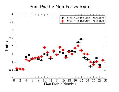
- 0.a.) Table .
| Pion Paddle Number | error | |
| 1 | 0.52 | 0.00188670 |
| 2 | 0.56 | 0.00075818 |
| 3 | 0.55 | 0.00080325 |
| 4 | 1.31 | 0.00152123 |
| 5 | 1.44 | 0.00158249 |
| 6 | 1.18 | 0.00084919 |
| 7 | 1.26 | 0.00096229 |
| 8 | 1.19 | 0.00066468 |
| 9 | 1.12 | 0.00077990 |
| 10 | 1.5 | 0.00113494 |
| 11 | 1.45 | 0.00137556 |
| 12 | 1.22 | 0.00070398 |
| 13 | 1.65 | 0.00147872 |
| 14 | 1.47 | 0.00122783 |
| 15 | 1.63 | 0.00154233 |
| 16 | 1.57 | 0.00162007 |
| 17 | 1.38 | 0.00138704 |
| 18 | 1.68 | 0.00288459 |
| 19 | 1.68 | 0.00321234 |
| 20 | 1.65 | 0.00394896 |
| 21 | 2.23 | 0.00993885 |
| 22 | 2.42 | 0.01726570 |
| 23 | 1.29 | 0.00877380 |
| 24 | 1.17 | 0.00650948 |
| 25 | 0.74 | 0.00280451 |
| 26 | 1 | 0.00808644 |
| 27 | 1.25 | 0.01073753 |
| 28 | 0.84 | 0.00615573 |
| 29 | 1.11 | 0.00957284 |
- 0.b.) Table .
| Pion Paddle Number | error | |
| 1 | 0.61 | 0.00136217 |
| 2 | 0.58 | 0.00072875 |
| 3 | 0.56 | 0.00063600 |
| 4 | 1.16 | 0.00084147 |
| 5 | 1.09 | 0.00067329 |
| 6 | 1.22 | 0.00084552 |
| 7 | 1.26 | 0.00077718 |
| 8 | 1.3 | 0.00071299 |
| 9 | 1.35 | 0.00095814 |
| 10 | 1.91 | 0.00150046 |
| 11 | 1.6 | 0.00131397 |
| 12 | 1.32 | 0.00072210 |
| 13 | 1.71 | 0.00129895 |
| 14 | 1.46 | 0.00093334 |
| 15 | 1.93 | 0.00219770 |
| 16 | 1.76 | 0.00160711 |
| 17 | 1.29 | 0.00106561 |
| 18 | 1.63 | 0.00205808 |
| 19 | 1.49 | 0.00210549 |
| 20 | 1.87 | 0.00366838 |
| 21 | 2.01 | 0.00692445 |
| 22 | 1.73 | 0.00746426 |
| 23 | 1.51 | 0.00978854 |
| 24 | 1.5 | 0.00801872 |
| 25 | 1.01 | 0.00349049 |
| 26 | 0.86 | 0.00424348 |
| 27 | 1.04 | 0.00729985 |
| 28 | 0.69 | 0.00620402 |
| 29 | 1.12 | 0.01390308 |
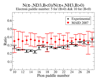
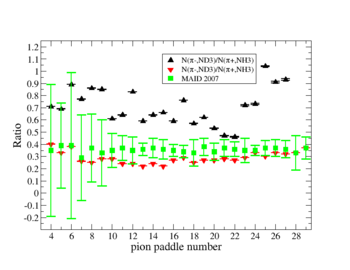
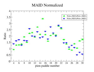
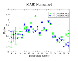
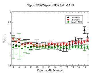
Perhaps we see if the MAID model can tell us what this ratio should be
Media:NH3positivepionMAID.pdfMedia:ND3negativepionMAID.pdf
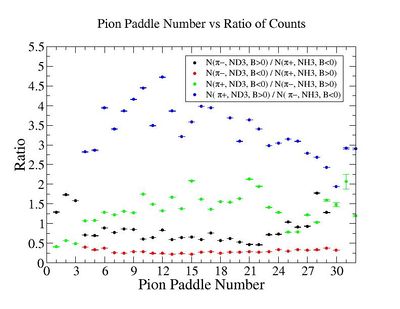
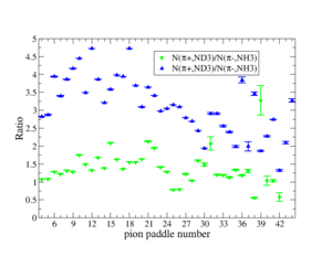
- 1.) Table 1.
| Pion Paddle Number | error | |||
| 1 | 77 | 65 | 0.4075770 | 0.0009842584 |
| 2 | 159 | 97 | 0.5639721 | 0.0006539302 |
| 3 | 149 | 105 | 0.4882354 | 0.0005272353 |
| 4 | 393 | 126 | 1.0731347 | 0.0007711509 |
| 5 | 444 | 141 | 1.0834182 | 0.0006573745 |
| 6 | 484 | 130 | 1.2809561 | 0.0008725428 |
| 7 | 496 | 140 | 1.2189500 | 0.0007440855 |
| 8 | 578 | 151 | 1.3169920 | 0.0007160697 |
| 9 | 471 | 127 | 1.2759964 | 0.0009002428 |
| 10 | 599 | 118 | 1.7465341 | 0.0013677534 |
| 11 | 497 | 115 | 1.4869309 | 0.0012131589 |
| 12 | 582 | 151 | 1.3261062 | 0.0007208959 |
| 13 | 588 | 121 | 1.6719536 | 0.0012616248 |
| 14 | 546 | 136 | 1.3812936 | 0.0008776225 |
| 15 | 558 | 92 | 2.0867894 | 0.0023701069 |
| 16 | 505 | 107 | 1.6238274 | 0.0014740763 |
| 17 | 454 | 115 | 1.3582830 | 0.0011103103 |
| 18 | 388 | 86 | 1.5522638 | 0.0019569046 |
| 19 | 359 | 80 | 1.5439624 | 0.0021696589 |
| 20 | 304 | 64 | 1.6342777 | 0.0032068058 |
| 21 | 272 | 44 | 2.1269069 | 0.0073027548 |
| 22 | 215 | 38 | 1.9466466 | 0.0083331144 |
| 23 | 119 | 29 | 1.4118261 | 0.0091055132 |
| 24 | 123 | 33 | 1.2823997 | 0.0068297700 |
| 25 | 102 | 45 | 0.7798659 | 0.0026920919 |
| 26 | 82 | 36 | 0.7836887 | 0.0037785779 |
| 27 | 99 | 28 | 1.2164924 | 0.0083029104 |
| 28 | 75 | 25 | 1.0321754 | 0.0084089279 |
| 29 | 88 | 19 | 1.5935340 | 0.0193377338 |
| 30 | 43 | 10 | 1.4794514 | 0.0470776577 |
| 31 | 30 | 5 | 2.0643508 | 0.1850680665 |
| 32 | 59 | 17 | 1.1940853 | 0.0172383351 |
| 33 | 83 | 24 | 1.1898689 | 0.0102416449 |
| 34 | 85 | 26 | 1.1248065 | 0.0086048876 |
| 35 | 93 | 24 | 1.3332266 | 0.0114363482 |
| 36 | 79 | 23 | 1.1817660 | 0.0108450951 |
| 37 | 34 | 9 | 1.2997764 | 0.0485842596 |
| 38 | 32 | 20 | 0.5504936 | 0.0068650227 |
| 39 | 38 | 4 | 3.2685555 | 0.4088076301 |
| 40 | 12 | 4 | 1.0321754 | 0.1313894981 |
| 41 | 30 | 10 | 1.0321754 | 0.0332392060 |
| 42 | 5 | 3 | 0.5734308 | 0.1216930868 |
- 2.) Table 2.
| paddleNumber | error | |||
| 1 | 59 | 5 | 30.21 | 2.70258040 |
| 2 | 79 | 14 | 14.45 | 0.27652327 |
| 3 | 73 | 8 | 23.36 | 1.03300637 |
| 4 | 65 | 59 | 2.82 | 0.00822726 |
| 5 | 55 | 49 | 2.87 | 0.01094524 |
| 6 | 80 | 52 | 3.94 | 0.01185748 |
| 7 | 65 | 49 | 3.4 | 0.01183225 |
| 8 | 113 | 75 | 3.86 | 0.00675056 |
| 9 | 117 | 72 | 4.16 | 0.00756073 |
| 10 | 200 | 115 | 4.45 | 0.00393821 |
| 11 | 226 | 166 | 3.49 | 0.00192550 |
| 12 | 328 | 178 | 4.72 | 0.00213914 |
| 13 | 391 | 259 | 3.86 | 0.00105330 |
| 14 | 360 | 287 | 3.21 | 0.00081064 |
| 15 | 389 | 278 | 3.58 | 0.00090286 |
| 16 | 426 | 274 | 3.98 | 0.00098738 |
| 17 | 437 | 284 | 3.94 | 0.00092912 |
| 18 | 444 | 241 | 4.72 | 0.00135761 |
| 19 | 419 | 291 | 3.69 | 0.00085791 |
| 20 | 397 | 329 | 3.09 | 0.00064841 |
| 21 | 407 | 286 | 3.64 | 0.00087414 |
| 22 | 346 | 260 | 3.41 | 0.00096976 |
| 23 | 274 | 235 | 2.98 | 0.00105807 |
| 24 | 430 | 361 | 3.05 | 0.00056086 |
| 25 | 478 | 388 | 3.15 | 0.00051121 |
| 26 | 471 | 390 | 3.09 | 0.00050259 |
| 27 | 420 | 385 | 2.79 | 0.00049185 |
| 28 | 342 | 326 | 2.69 | 0.00062326 |
| 29 | 266 | 280 | 2.43 | 0.00076396 |
| 30 | 78 | 103 | 1.94 | 0.00337017 |
| 31 | 33 | 29 | 2.91 | 0.02416684 |
| 32 | 34 | 30 | 2.9 | 0.02293226 |
| 33 | 32 | 32 | 2.56 | 0.01999906 |
| 34 | 28 | 30 | 2.39 | 0.02171314 |
| 35 | 17 | 22 | 1.98 | 0.03411592 |
| 36 | 21 | 14 | 3.84 | 0.08345855 |
| 37 | 7 | 9 | 1.99 | 0.13036518 |
| 38 | 27 | 20 | 3.46 | 0.04582149 |
| 39 | 24 | 33 | 1.86 | 0.01863261 |
| 40 | 31 | 35 | 2.27 | 0.01710150 |
| 41 | 76 | 71 | 2.74 | 0.00617114 |
| 42 | 16 | 31 | 1.32 | 0.02201769 |
| 43 | 18 | 22 | 2.09 | 0.03411970 |
| 44 | 23 | 18 | 3.27 | 0.05209530 |
- 3.) Table 3.
| Pion Paddle Number | error | ||
| 0.91 | 45 | 89 | 1.29 0.004556 |
| 1.91 | 86 | 127 | 1.73 0.002488 |
| 2.91 | 82 | 133 | 1.58 0.002361 |
| 3.91 | 91 | 330 | 0.71 0.000822 |
| 4.91 | 94 | 348 | 0.69 0.000766 |
| 5.91 | 125 | 360 | 0.89 0.000649 |
| 6.91 | 120 | 399 | 0.77 0.000594 |
| 7.91 | 148 | 443 | 0.86 0.000484 |
| 8.91 | 128 | 387 | 0.85 0.000595 |
| 9.91 | 121 | 510 | 0.61 0.000459 |
| 10.91 | 104 | 417 | 0.64 0.000607 |
| 11.91 | 145 | 449 | 0.83 0.000481 |
| 12.91 | 108 | 469 | 0.59 0.000528 |
| 13.91 | 113 | 449 | 0.64 0.000541 |
| 14.91 | 104 | 401 | 0.66 0.000631 |
| 15.91 | 98 | 427 | 0.59 0.000609 |
| 16.91 | 100 | 335 | 0.76 0.000774 |
| 17.91 | 70 | 316 | 0.57 0.000973 |
| 18.91 | 65 | 269 | 0.62 0.001189 |
| 19.91 | 56 | 270 | 0.53 0.001273 |
| 20.91 | 37 | 200 | 0.47 0.002111 |
| 21.91 | 27 | 149 | 0.46 0.003316 |
| 22.91 | 28 | 99 | 0.72 0.004942 |
| 23.91 | 32 | 112 | 0.73 0.004087 |
| 24.91 | 42 | 103 | 1.04 0.003963 |
| 25.91 | 25 | 70 | 0.91 0.007479 |
| 26.91 | 24 | 66 | 0.93 0.008105 |
| 27.91 | 27 | 39 | 1.77 0.014578 |
| 28.91 | 24 | 48 | 1.28 0.011546 |
- 4.) Table 4.
| Pion Paddle Number | error | ||
| 3.89 | 81 | 69 | 0.4 0.000896 |
| 4.89 | 84 | 87 | 0.33 0.000595 |
| 5.89 | 84 | 76 | 0.38 0.000757 |
| 6.89 | 75 | 98 | 0.26 0.000488 |
| 7.89 | 91 | 123 | 0.25 0.000348 |
| 8.89 | 115 | 141 | 0.28 0.000283 |
| 9.89 | 207 | 254 | 0.28 0.000117 |
| 10.89 | 212 | 300 | 0.24 0.000092 |
| 11.89 | 284 | 413 | 0.24 0.000057 |
| 12.89 | 322 | 501 | 0.22 0.000043 |
| 13.89 | 359 | 521 | 0.24 0.000040 |
| 14.89 | 365 | 565 | 0.22 0.000036 |
| 15.89 | 415 | 523 | 0.27 0.000040 |
| 16.89 | 444 | 526 | 0.29 0.000039 |
| 17.89 | 405 | 555 | 0.25 0.000036 |
| 18.89 | 414 | 528 | 0.27 0.000039 |
| 19.89 | 387 | 502 | 0.27 0.000042 |
| 20.89 | 408 | 505 | 0.28 0.000042 |
| 21.89 | 352 | 457 | 0.27 0.000048 |
| 22.89 | 298 | 358 | 0.29 0.000070 |
| 23.89 | 522 | 547 | 0.33 0.000038 |
| 24.89 | 530 | 608 | 0.3 0.000032 |
| 25.89 | 571 | 590 | 0.33 0.000034 |
| 26.89 | 523 | 564 | 0.32 0.000036 |
| 27.89 | 422 | 440 | 0.33 0.000052 |
| 28.89 | 368 | 342 | 0.37 0.000079 |
| 29.89 | 101 | 108 | 0.32 0.000427 |
Corrected one just has values of 1.
2.) Kinematic plots for all 8 conditions
4/4/11
1.) Document the electron efficiency -vs- paddle ( for each target separately) and pion efficiency -vs- paddle in thesis
| Inclusive detected electrons -vs- Q-squared |
*Inclusive
Media:ND3andNH3electronpaddlenumberinclusive.pdf
Media:NH3Q2inclusive.pdfMedia:ND3Q2inclusive.pdf
- Semi Inclusive
Media:ND3electronpaddlenumbersemi_inclusive.pdfMedia:NH3electronpaddlenumbersemi_inclusive.pdf
2.) Compare to MAI2007 for paddles with unity pion efficiency ratios
Total Cross Section:
where
is pion azimuthal angle in CM frame, - virtual photon polarization.
where , (the difference between the initial and final energy of the electron).
- Four momentum transferred square.
- electron scattering angle.
h - electron helicity.
where
Media:NH3positivepionMAID.pdfMedia:ND3negativepionMAID.pdf
5/11/11
1.) Document the electron efficiency -vs- paddle ( for each target separately) and pion efficiency -vs- paddle in thesis
Zoom in on the Q^2 range from 0.9 to 1.3 fine binning.
2.) Media:X_BEpaddlenumber5and10.pdf
3.)
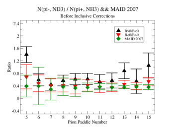
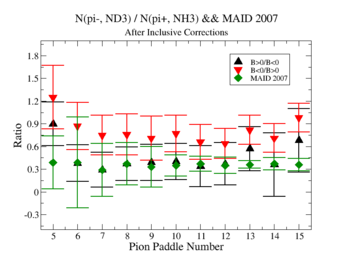
MAID is the dominant error? The data agree with MAID statistically.
Yes it is.
5/23/11
1.) Detector is not working. Two GEM foils are packed for shipping. The current measured across the GEM Foils at ~120 Volts is 1-5 nAmp.
Media:theorynd3bn_nh3bp_ratio.pdf
5/25/11
In this case, corrections from the inclusive data are applied.
6/27/11
1.) Analyze data for asymmetries.
a.) Charge asymmetry -vs- run number plot
b.) Rate sums and difference plots i.) Insert histogram names here and their definitions
2.)Histograms for error calculation
3.) Dilution factor histogram names and definition
07/23/11
Make it easier to see the differences.  Subtract experiment from Maid2007 and put
the before and after corrections results on the same graph.
Use different error bars for the error from the correction factor
and the statistical uncertainties (1/sqrt(N).
Exclusive cases
07/28/11
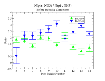
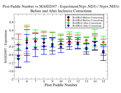
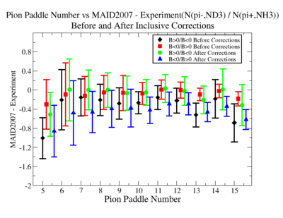
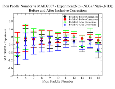
- 1.) Pion Paddle number vs ratio for MAID2007-Experiment :
You need to make the above graph in black and white then it will be ready for your thesis.
This means you need to change the error bars so you can identify them when they
are in black and white.
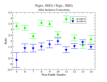
- I would conclude from the above that the correction does not impact inclusive single pion production while it does make the semi-inclusive data less dependent on Torus polarity.
You should add the systematic error as a separate uncertainty to the graph.
Usually you can remove the riser from the larger uncertainty and include the riser (the horizontal bar) on the smaller uncertainty..
- 2.) Charge Asymmetry:
You have a choice for the charge asymmetry, either do a linear fit to run number
or average over all runs.  I prefer averaging over all runs and displaying it as a
histogram for the data set to measure false asymmetries from the beam alone
ND3Bn
08/01/11
Charge Asymmetry
- 1). ND3Bp
- 2). NH3Bn
- 3). NH3Bp
Average charge(beam) Asymmetry:
Add some text describing the difference in the charge asymmetry plots.
I dont understand what makes the plot below so different from the ones above.
 File:ChargeAsymmetryNH3Bp 2.pdf
Calculating and
This calculation will contain many terms. It may be best to break it up into several parts.
9/30/11 DST copies from JLab
I copied the following from the JLab cache disk to isulinux1
outbending
scp /cache/mss/clas/eg1b/production/pass1/v4/4p2out/misc/dst/dst2828* isulinux1:/local/scratch/tforest/4.2negND3
scp /cache/mss/clas/eg1b/production/pass1/v4/4p2out/misc/dst/dst283* isulinux1:/local/scratch/tforest/4.2negND3
scp /cache/mss/clas/eg1b/production/pass1/v4/4p2out/misc/dst/dst2829* isulinux1:/local/scratch/tforest/4.2negND3
scp /cache/mss/clas/eg1b/production/pass1/v4/4p2out/misc/dst/dst284* isulinux1:/local/scratch/tforest/4.2negNH3
in bending
scp /w/cache/mss/home/nguler/dst/dst282* isulinux1:/local/scratch/tforest/4.2PosNH3
scp /w/cache/mss/home/nguler/dst/dst281* isulinux1:/local/scratch/tforest/4.2PosND3
10/7/11 sftp file copying
Another way to copy files from JLab is to copy them from the /cache disk to the /u/scratch disk and then sftp them from JLab.
sftp username@ftp.jlab.org
cd /u/scratch/tforest
mget *
12/16/11
Charge Asymmetry
01/30/12
Charge Asymmetry
In double spin asymmetry measurements it is important to eliminate any source of false asymmetry, like charge asymmetry. The helicity of the electron beam was flipped with a rate of 1 HZ and its original state was chosen at the injector in a pseudo-random way. The next state of the electron helicity, so called complement state, is always with opposite helicity. The diagram on Fig. 3.1 represents the helicity state.
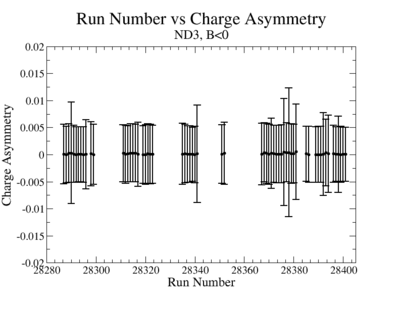
A one bit signal from the beam injector gives the helicity information, whereas a sync bit with a 2 HZ frequency is generated at the same time and is equal to the helicity flip time. However, the electron beam helicity sequence can be interrupted by the Data Acquisition System(DAQ), like leaving unpaired helicity states and dead time problems. In order to eliminate the asymmetry caused by the DAQ, the Faraday cup was installed to measure the charge simultaneously with the helicity state flip. The stored data files include accumulated charge value for each helicity state. The measured charge asymmetry is shown bellow for 4.2 GeV data that has been collected for ND3 target while torus magnetic field was negative.
lifetime only takes data when daq is ready.
|
Figure 3.2. Run Number vs Charge Asymmetry (ND3 target, B<0) |
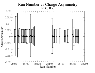
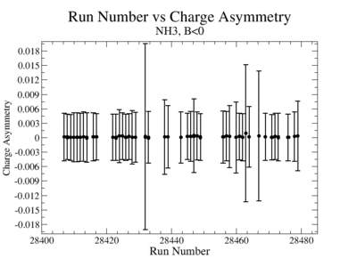
The charge asymmetry measured for each run number, thats is used for this analysis is shown on Fig. 3.3.
|
|
|
Figure 3.2. Run Number vs Charge Asymmetry for All Runs |
Charge Asym no sign correction
The uncertainty should be the same for the (1-4) and (2-3) distributions in the same run group. Use 12 groups of files (slugs) to create a histogram of the asymemtry and fit it with a gaussian.
Inclusive asymmetry as a function of X_B for all is shown on Fig. 3.4. The electron paddle numbers 10 and 5 were chosen respectively for B<0 and B>0, because they contained the most electron events in a first pass semi-inclusive pion analysis of the data set.
inclusive includes sign correction
For inclusive do run number vs inclusive Asymmetry
|
Figure 3.4. X_{bjorken} vs Inclusive Asymmetry(All data) |
02/06/12
Charge Asymmetry
In double spin asymmetry measurements it is important to eliminate any source of false asymmetry, like charge asymmetry. The helicity of the electron beam was flipped with a rate of 1 HZ and its original state was chosen at the injector in a pseudo-random way. The next state of the electron helicity, so called complement state, is always with opposite helicity. The diagram on Fig. 3.1 represents the helicity state.
A one bit signal from the beam injector gives the helicity information, whereas a sync bit with a 2 HZ frequency is generated at the same time and is equal to the helicity flip time. However, the electron beam helicity sequence can be interrupted by the Data Acquisition System(DAQ), like dead time problems. In order to eliminate the asymmetry caused by the DAQ, the Faraday cup was installed to measure the charge simultaneously with the helicity state flip. The stored data files include accumulated charge value for each helicity state. The measured charge asymmetry is shown bellow for 4.2 GeV data that has been collected for ND3 target while torus magnetic field was negative.
|
Figure 3.2. Run Number vs Charge Asymmetry (ND3 target, B<0) |
The charge asymmetry measured for each run number, thats is used for this analysis is shown on Fig. 3.3.
|
|
|
Figure 3.2. Run Number vs Charge Asymmetry for All Runs |
Inclusive asymmetry as a function of X_B for all is shown on Fig. 3.4. The electron paddle numbers 10 and 5 were chosen respectively for B<0 and B>0, because they contained the most electron events in a first pass semi-inclusive pion analysis of the data set.
|
Figure 3.4. X_{bjorken} vs Inclusive Asymmetry(All data) |
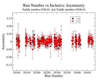
The Figures 3.5 and 3.6 show inclusive asymmetry for each run number and for run groups used for these analysis
|
Figure 3.5. Run Number vs Inclusive Asymmetry |
|
Figure 3.5. Run groups vs Inclusive Asymmetry |
03/06/12
NES Asymmetry
The double spin asymmetry measurements performed in this thesis are performed by comparing scattering events that occur when the incident probe spin and nuclear target spin are parallel to scattering events that occur when the spins are anti-parallel. The helicity of the electron beam was flipped at a rate of 1 HZ. The helicity is prepared at the source such that helicity pairs are produced pseudo randomly. If the first electron bunch is pseudo randomly chosen to be positive (negative) then it is labeled as the original helicity state and denoted in software by a 2 (1). The next helicity state is prepared to be a complement to the first state and labeled in the software as either a 4, if the original helicity state was a 1 (negative), or 3 if the original helicity state was a 2 (positive). The helicity process is then repeated. Figure NES.1 illustrates the signals used to label helicity state. The clock pulse (SYNC) is used to indicate that a change in the pockel cell used to define the helicity state may have occurred. The helicity bit indicates the helicity state that was set. The original/complement pulse identifies if the state is an original or complement helicity state. All three bits are recorded in the raw data file for each event and then converted to the labels 1,2,3,4 during DST file production once the particles have been reconstructed.
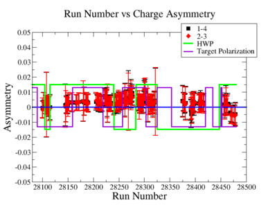
Two scalers were used to record several ancillary detectors, such as a Faraday cup and several PMTs mounted on the beam line, according to their helicity label. One of the scalers was gated by the DAQ live time in order to record beam conditions when the DAQ was able to take data and not busy recording data. The second scaler remained ungated. Both scalers recorded the SYNC and Helicity signals from the injector along with the counts observed from ancillary detectors during the SYNC interval. The Faraday cup signal recorded by the gated helicity scaler is used to normalize the events reconstructed during the same helicity interval. The beam charge asymmetry measured by the gated helicity scaler is shown in Figure NES. 2. as a function of run number. For each run number the gaussian fit was used to extract the mean values of the asymmetry and corresponding error(Figure NES. 3).
|
Figure NES. 2. Run Number vs the beam charge Asymmetry |
|
Figure NES. 3. Beam charge asymmetry for run #28101 using the gated faraday cup counts for two helicity pairs(1-4 and 2-3 helicity pairs). and |
| Run Group | Half wave plane(HWP) | ||
| 28100 - 28105 | +1 | ||
| 28106 - 28115 | -1 | ||
| 28145 - 28240 | +1 | ||
| 28242 - 28284 | -1 | ||
| 28286 - 28324 | +1 | ||
| 28325 - 28447 | -1 | ||
| 28449 - 28479 | +1 |
A measurement of the electron cross section helicity difference needs to account for the possible helicity dependence of the incident electron flux ( Charge Asymmetry). Fig. NES. 4 shows the reconstructed electron asymmetry before it is normalized by the gated Faraday Cup as a function of the run number for the 4.2 GeV data set. The reconstructed electron asymmetry can be defined following way:
- or
where () represents number of reconstructed electrons in the final state for the positive(negative) beam helicity.
|
Figure NES.4. Run Number vs NES Asymmetry for All Runs before FC normalization |
Sysstematic effects on the asymmetry measurement may be investigated by separating the data into two groups based on which helicity state is set first. The first group(black data points) represents the electron asymmetry observed when the first (original) helicity state is negative and its complement state is positive(helicity state #1 - state #4). The second group(red data points) represents the asymmetry observed, when the first state is positive and the complement state is negative(helicity state #2 - #3). Both groups were divided into two subgroups based the target type used. The diamond points on the histogram represent the data for the NH3 target and the squares for the ND3 target. On the same histograms are presented the signs of the half wave plane(HWP) and the target polarization(TPol). The relative spin orientation can be changed by either inserting a half wave (HWP) or by populating a different target polarization state with a different RF frequency. One would expect the asymmetry to change sign if either the HWP is inserted or the target polarization is rotated 180 degrees. As one can see, the electron asymmetry sign ( sign(hel1-hel4) && sign(hel3-hel2) ) is opposite of the sign of (HWPTarget_Polarization). The NES asymmetry has been calculated the following way before accounting for the Faraday cup:
The NES asymmetry after the gated faraday cup normalization is defined as:
|
Figure NES.5. Run Number vs NES Asymmetry for All Runs after FC normalization |
On the Fig. NES. 6 data runs are combined for the same target type, target polarization, beam torus and half wave plane.
|
Figure NES. 6. Run groups vs NES Asymmetry before and after FC Normalization |
03/12/12
SIDIS Asymmetry
SIDIS asymmetries:
|
|
|
|
|
Figure NES. 6. Run Number vs Semi inclusive asymmetry before FC Normalization. |
|
Figure NES. 6. Run Number vs Semi inclusive asymmetry after FC Normalization. |
| Target type, Beam Torus sign (B) | |||
| NH3, B>0, | |||
| NH3, B<0, | |||
| ND3, B>0, | |||
| ND3, B<0, | |||
| NH3, B>0, | |||
| NH3, B<0, | |||
| ND3, B>0, | |||
| ND3, B<0, |
| Run Group | Target type, Beam Torus sign (B) | A_{1-4} | A_{2-3} |
| 28214 - | NH3, B>0 | 0.02399480 \pm 0.01700174 | |
| 28231 - | NH3, B>0 | -0.01372286
\pm 0.01559729 | |
| 28252 - | NH3, B>0 | -0.00048034 \pm 0.01685103 | |
| 28266 - | NH3, B>0 | -0.02002048 \pm 0.01610756 | |
| 28413 - | NH3, B<0 | 0.02205009 \pm 0.01799869 | -0.02291024 \pm 0.01795956 |
| 28469 - | NH3, B<0 | 0.02270121 \pm 0.01543980 | -0.02662038 \pm 0.01532731 |
| 28102 - | ND3, B>0 | 0.04443768 \pm 0.06093347 | 0.01055158 \pm 0.06066387 |
| 28109 - | ND3, B>0 | 0.01068017 \pm 0.03953670 | -0.00764924 \pm 0.03970762 |
| 28150 - | ND3, B>0 | -0.01238850 \pm 0.03640693 | 0.02901657 \pm 0.03642766 |
| 28182 - | ND3, B>0 | -0.02497960 \pm 0.02660287 | 0.00797540 \pm 0.02634698 |
| 28295 - | ND3, B<0 | -0.01323095 \pm 0.01636848 | -0.01008145 \pm 0.01636433 |
| 28315 - | ND3, B<0 | -0.01026453 \pm 0.01768742 | 0.00621953 \pm 0.01758502 |
| 28393 - | ND3, B<0 | 0.01615151 \pm 0.01853525 | -0.00719786 \pm 0.01834110 |
|
Figure NES. 6. Run groups vs Semi inclusive asymmetry after FC Normalization. |
X and Z count distribution
| SIDI Asymmetry | ||
| 0.3 | ||
| 0.5 | ||
| 0.7 | ||
| 0.9 |
| 0.45 | ||
| 0.7 | ||
| 0.9 |
| 0.3 | ||
| 0.5 | ||
| 0.7 | ||
| 0.9 |
"If each observable () is accompanied by an estimate of the uncertainty in that observable () then the weighted mean is defined as
- "
"The variance of the distribution is defined as
- = weighted variance"
| 0.3 | ||
| 0.5 | ||
| 0.7 | ||
| 0.9 |
| Table 4.5. Experimental Results of The Fragmentation Function vs and for four values of . |
| 0.45 | ||
| 0.85 |
| Table 4.6. Experimental Results of The Fragmentation Function vs and (Combined ). |
| 0.8 | 2.4 | 0.344712 | 0.089457 | 1.215956 |
| 0.8 | 2.56 | 0.322805 | 0.087636 | 1.144319 |
| 0.8 | 2.72 | 0.302941 | 0.087324 | 1.142601 |
| 0.8 | 2.89 | 0.284872 | 0.080418 | 1.081259 |
| 0.8 | 3.06 | 0.268386 | 0.046144 | 0.971948 |
| 0.8 | 3.24 | 0.253303 | -0.001413 | 0.904000 |
| 0.8 | 3.42 | 0.239465 | -0.039615 | 0.888457 |
| 0.85 | 2.4 | 0.358532 | 0.095124 | 1.179011 |
| 0.85 | 2.56 | 0.336197 | 0.092376 | 1.118478 |
| 0.85 | 2.72 | 0.315894 | 0.091414 | 1.126200 |
| 0.85 | 2.89 | 0.297382 | 0.083684 | 1.073062 |
| 0.85 | 3.06 | 0.280456 | 0.047397 | 0.965145 |
| 0.85 | 3.24 | 0.264940 | 0.000751 | 0.897095 |
| 0.85 | 3.42 | 0.250680 | -0.037185 | 0.879470 |
| 0.9 | 2.4 | 0.371781 | 0.101758 | 1.124929 |
| 0.9 | 2.56 | 0.349070 | 0.097293 | 1.077209 |
| 0.9 | 2.72 | 0.328374 | 0.095640 | 1.097502 |
| 0.9 | 2.89 | 0.309461 | 0.087175 | 1.064119 |
| 0.9 | 3.06 | 0.292134 | 0.050127 | 0.968564 |
| 0.9 | 3.24 | 0.276219 | 0.003136 | 0.902680 |
| 0.9 | 3.42 | 0.261569 | -0.034673 | 0.882556 |
| 0.95 | 2.4 | 0.384494 | 0.107726 | 1.079087 |
| 0.95 | 2.56 | 0.361453 | 0.102269 | 1.040995 |
| 0.95 | 2.72 | 0.340407 | 0.099848 | 1.072015 |
| 0.95 | 2.89 | 0.321133 | 0.090544 | 1.055804 |
| 0.95 | 3.06 | 0.303439 | 0.052833 | 0.971023 |
| 0.95 | 3.24 | 0.287158 | 0.005393 | 0.907107 |
| 0.95 | 3.42 | 0.272146 | -0.032200 | 0.884625 |
| 1 | 2.4 | 0.396703 | 0.113466 | 1.036707 |
| 1 | 2.56 | 0.373374 | 0.106727 | 1.007923 |
| 1 | 2.72 | 0.352016 | 0.103726 | 1.047463 |
| 1 | 2.89 | 0.332416 | 0.093605 | 1.045933 |
| 1 | 3.06 | 0.314388 | 0.055305 | 0.970792 |
| 1 | 3.24 | 0.297772 | 0.007453 | 0.909048 |
| 1 | 3.42 | 0.282424 | -0.029966 | 0.884723 |
| 1.05 | 2.4 | 0.408437 | 0.118939 | 0.992592 |
| 1.05 | 2.56 | 0.384858 | 0.111105 | 0.971331 |
| 1.05 | 2.72 | 0.363224 | 0.107103 | 1.019267 |
| 1.05 | 2.89 | 0.343330 | 0.095852 | 1.029986 |
| 1.05 | 3.06 | 0.324999 | 0.057266 | 0.964081 |
| 1.05 | 3.24 | 0.308073 | 0.009820 | 0.906637 |
| 1.05 | 3.42 | 0.292416 | -0.027198 | 0.883994 |
| 1.1 | 2.4 | 0.419723 | 0.125251 | 0.947155 |
| 1.1 | 2.56 | 0.395929 | 0.115416 | 0.938049 |
| 1.1 | 2.72 | 0.374051 | 0.110297 | 0.993433 |
| 1.1 | 2.89 | 0.353894 | 0.098076 | 1.014245 |
| 1.1 | 3.06 | 0.335286 | 0.059359 | 0.956429 |
| 1.1 | 3.24 | 0.318077 | 0.012982 | 0.905373 |
| 1.1 | 3.42 | 0.302133 | -0.024350 | 0.882958 |
| 1.15 | 2.4 | 0.430586 | 0.130979 | 0.910430 |
| 1.15 | 2.56 | 0.406608 | 0.119423 | 0.907506 |
| 1.15 | 2.72 | 0.384515 | 0.113163 | 0.969323 |
| 1.15 | 2.89 | 0.364122 | 0.100019 | 0.998793 |
| 1.15 | 3.06 | 0.345265 | 0.061046 | 0.948539 |
| 1.15 | 3.24 | 0.327796 | 0.015164 | 0.901680 |
| 1.15 | 3.42 | 0.311587 | -0.021709 | 0.880861 |
| 1.2 | 2.4 | 0.441050 | 0.136174 | 0.877989 |
| 1.2 | 2.56 | 0.416916 | 0.123376 | 0.879867 |
| 1.2 | 2.72 | 0.394636 | 0.116022 | 0.947092 |
| 1.2 | 2.89 | 0.374032 | 0.101867 | 0.984262 |
| 1.2 | 3.06 | 0.354948 | 0.062766 | 0.940538 |
| 1.2 | 3.24 | 0.337242 | 0.017174 | 0.897860 |
| 1.2 | 3.42 | 0.320789 | -0.019216 | 0.878344 |
| 1.25 | 2.4 | 0.451137 | 0.141522 | 0.851328 |
| 1.25 | 2.56 | 0.426872 | 0.127836 | 0.854448 |
| 1.25 | 2.72 | 0.404429 | 0.119066 | 0.924399 |
| 1.25 | 2.89 | 0.383638 | 0.104151 | 0.966286 |
| 1.25 | 3.06 | 0.364349 | 0.064626 | 0.929040 |
| 1.25 | 3.24 | 0.346426 | 0.019518 | 0.890588 |
| 1.25 | 3.42 | 0.329748 | -0.016436 | 0.873707 |
| 1.3 | 2.4 | 0.460866 | 0.146979 | 0.827067 |
| 1.3 | 2.56 | 0.436494 | 0.131843 | 0.832123 |
| 1.3 | 2.72 | 0.413910 | 0.122206 | 0.903273 |
| 1.3 | 2.89 | 0.392954 | 0.106218 | 0.949548 |
| 1.3 | 3.06 | 0.373480 | 0.066537 | 0.917721 |
| 1.3 | 3.24 | 0.355358 | 0.021675 | 0.883594 |
| 1.3 | 3.42 | 0.338473 | -0.013711 | 0.868901 |
| 1.35 | 2.4 | 0.470256 | 0.151920 | 0.806259 |
| 1.35 | 2.56 | 0.445798 | 0.135925 | 0.812231 |
| 1.35 | 2.72 | 0.423094 | 0.125351 | 0.884403 |
| 1.35 | 2.89 | 0.401992 | 0.108521 | 0.933955 |
| 1.35 | 3.06 | 0.382352 | 0.068511 | 0.907321 |
| 1.35 | 3.24 | 0.364050 | 0.023938 | 0.877039 |
| 1.35 | 3.42 | 0.346974 | -0.011047 | 0.864389 |
| Table 4.7. . |
| , | 0.006584 | 0.004943 |
| , | 0.006382 | 0.004355 |
| , | 0.005769 | 0.004544 |
| , | 0.005856 | 0.004021 |
| , | 0.002893 | 0.002574 |
| , | 0.001664 | 0.001361 |
| , | 0.002673 | 0.002399 |
| , | 0.001565 | 0.001307 |
| , | 0.00611464 | 0.00545206 |
| , | 0.00428864 | 0.00330646 |
| , | 0.00552027 | 0.00392858 |
| , | 0.00552027 | 0.00392858 |
| , | 0.00265003 | 0.00282080 |
| , | 0.00097612 | 0.00090184 |
| , | 0.00264221 | 0.00243020 |
| , | 0.00154130 | 0.00128547 |
| Table 4.7. Average . |
| 0.45 | ||
| 0.7 |
