Difference between revisions of "Wire angle correspondance"
| Line 8: | Line 8: | ||
<center>[[File:Wires_parallel_all_types.png]]</center> | <center>[[File:Wires_parallel_all_types.png]]</center> | ||
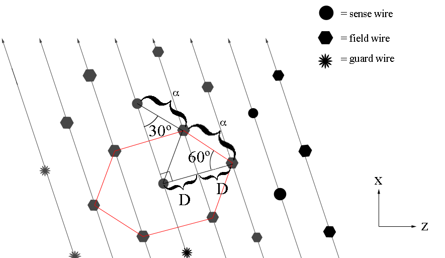
| − | Examining the geometry file, we can see that each plane, not just the plane of the sense wires, is separated by a distance of D=.3861 cm. Since each sensor wire is separated by four planes, the distance between two adjacent wires within a plane is given by | + | Examining the geometry file, we can see that each plane, not just the plane of the sense wires, is separated by a distance of D=.3861 cm. |
| + | |||
| + | <center>[[File:Hex.png]]</center> | ||
| + | |||
| + | |||
| + | Since each sensor wire is separated by four planes, the distance between two adjacent wires within a plane is given by | ||
Revision as of 04:55, 30 November 2016
Determining wire-theta correspondence
To associate the hits with the Moller scattering angle theta, the occupancy plots of the drift chamber hits by means of wire numbers and layer must be translated using the physical constraints of the detector. Using the data released for the DC:
DC: Drift Chambers(specs)
DC Geometry(geom)

Examining the geometry file, we can see that each plane, not just the plane of the sense wires, is separated by a distance of D=.3861 cm.

Since each sensor wire is separated by four planes, the distance between two adjacent wires within a plane is given by

CED Verification
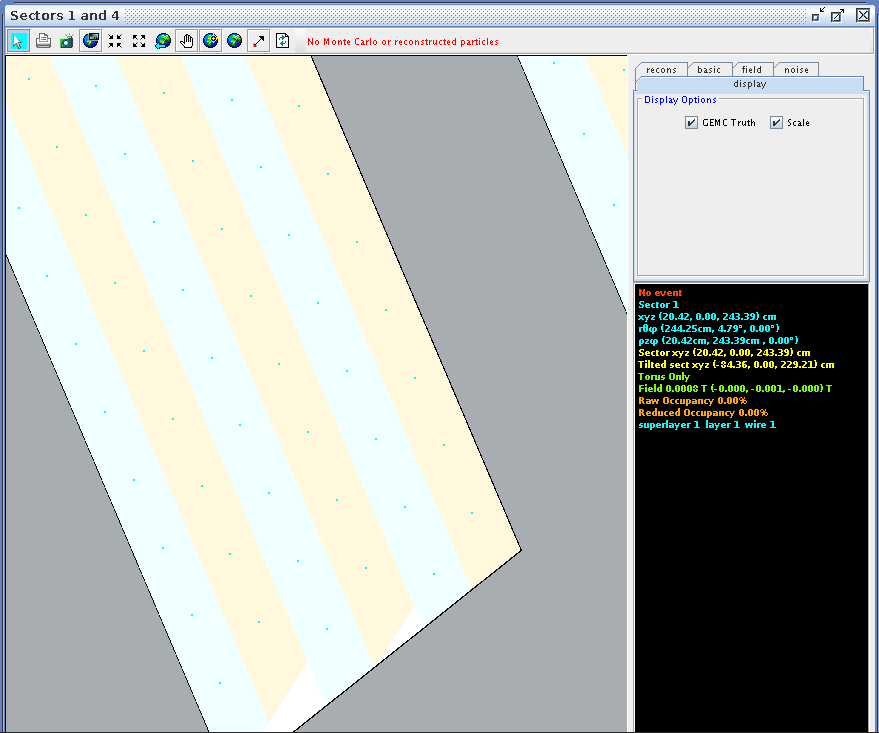
Using CED to verify the angle and wire correlation,
Zooming in on the view paralell to the direction of the wires in ced, we can examine the wire corresponding theta angle in the drift chamber.

Corresponding theta angles can be found for other wires, in Region 1, Superlayers 1 and 2.
| Wire Number | Layer 1 | Layer 2 | Layer 3 | Layer 4 | Layer 5 | Layer 6 |
|---|---|---|---|---|---|---|
| 1 | 4.79 | 5.03 | 4.98 | 5.22 | 5.16 | 5.40 |
| 2 | 5.09 | 5.33 | 5.27 | 5.51 | 5.45 | 5.69 |
| 77 | 29.46 | 29.60 | 29.41 | 29.55 | 29.37 | 29.51 |
| 78 | 29.79 | 29.93 | 29.74 | 29.88 | 29.69 | 29.83 |
| 79 | 30.12 | 30.26 | 30.07 | 30.21 | 30.02 | 30.16 |
| 110 | 40.19 | 40.28 | 40.05 | 40.13 | 39.91 | 39.99 |
| 111 | 40.51 | 40.59 | 40.36 | 40.44 | 40.21 | 40.29 |
| 112 | 40.82 | 40.90 | 40.67 | 40.75 | 40.52 | 40.60 |
| Wire Number | Layer 1 | Layer 2 | Layer 3 | Layer 4 | Layer 5 | Layer 6 |
|---|---|---|---|---|---|---|
| 1 | 4.79 | 5.03 | 4.98 | 5.22 | 5.16 | 5.40 |
| 2 | 5.09 | 5.33 | 5.27 | 5.51 | 5.45 | 5.69 |
| 77 | 29.46 | 29.60 | 29.41 | 29.56 | 29.37 | 29.51 |
| 78 | 29.79 | 29.93 | 29.74 | 29.88 | 29.70 | 29.84 |
| 79 | 30.13 | 30.27 | 30.07 | 30.21 | 30.02 | 30.16 |
| 110x | 40.19 | 40.28 | 40.05 | 40.13 | 39.91 | 39.99 |
| 111 | 40.51 | 40.59 | 40.36 | 40.44 | 40.22 | 40.30 |
| 112 | 40.82 | 40.90 | 40.67 | 40.75 | 40.52 | 40.60 |
Super Layer 1:Layer 1
Examing the range limits for the angle theta:
Taking the difference of the upper and lower limits in theta,
Dividing by the change in wire numbers (112-1=111), we find
This would imply that if the wires were evenly placed, their change in angle theta would increase by the factor of .325 degrees for each increase in wire number, starting obviously with wire 1 at 4.79 degrees. In addition, this implies that the bin spacing for each wire would be around .325 degrees in width.
Chercking this, we can find the difference between wires 1 and 2,
Similarly, finding the difference between wires 111 and 112,
These differing values show that the bin width is not uniform in length, therefore a linear fit will not suffice.
Changing cell size
Using Mathematica, a line can be fitted to the data collected on the wire number to angle theta correspondence.
Declaring the data set:
In[1]:= data1={{1,4.79},{2,5.09},{78,29.79},{111,40.50},{112,40.82}}

Out[1]= {{1,4.79},{2,5.09},{78,29.79},{111,40.5},{112,40.82}}
Testing for a linear fit:
In[2]:= line1=Fit[data1,{1,x},x]

Out[2]= 4.45395 +0.324738 x
Since the 1st deriviative of this function is not equal to the previous value of .3246 degrees, we will need to test the next order.
Testing for a quadratic fit:
In[3]:= quad1=Fit[data1,{1,x,x^2},x]

Out[3]= 4.45253 +0.325072 x-3.05048*10^-6 x^2
Testing for a polynomial of degree 3 fit:
In[118]:= polynomial1=Fit[data1,{1,x,x^2,x^3},x]

Out[118]= 4.48739 +0.300911 x+0.000510988 x^2-2.6919*10^-6 x^3