Difference between revisions of "VanWasshenova Thesis"
Jump to navigation
Jump to search
| Line 43: | Line 43: | ||
==Detector Occupancy== | ==Detector Occupancy== | ||
| + | ==Comparing Rates== | ||
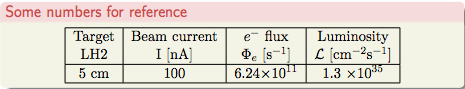
| + | Using the values from Whitney: | ||
| + | |||
| + | <center>[[File:Whitney_values.png]]</center> | ||
| + | |||
| + | For a 5cm target of LH2: | ||
| + | |||
| + | <center><math>\rho_{target}\times l_{target}=\frac{70.85 kg}{1 m^3}\times \frac{1 mole}{2.02 g} \times \frac{1000g}{1 kg} \times \frac{6.022\times10^{23} molecules\ LH_2}{1 mole} \frac{2 atoms}{1\ molecule\ LH_2} \times \frac{1m^3}{(100 cm)^3} \times \frac{5 cm}{ }=2.11\times 10^{23} \times \frac{10^{-24} cm^{2}}{barn}=2.11\times 10^{-1}\ barns^{-1}</math></center> | ||
| + | |||
| + | |||
| + | Using the beam current of 100nA, | ||
| + | |||
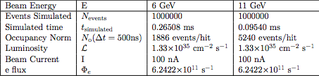
| + | <center><math>\Phi_{beam}=\frac{100\times 10^{-9}\ A}{1} \times \frac{1\ C}{1\ A} \times \frac{1\ e^{-}}{1\ s} \times \frac{1}{1.602\times 10^{-19}C}\Rightarrow 6.2422\times 10^{11}\ \frac{1}{s}=\Phi_{e^{-}}</math></center> | ||
| + | |||
| + | |||
| + | Given the beam Luminosity of: | ||
| + | <center><math>\mathcal {L}=\frac{1.32\times 10^{35}}{cm^2 \cdot s}\frac{10^{-24} cm^{2}}{barn}=\frac{1.32\times 10^{11}}{barn\cdot s}=\Phi_{beam}\ \rho\ l_{target}</math></center> | ||
| + | |||
| + | We can check to make sure the density makes sense | ||
| + | |||
| + | <center><math>\Rightarrow \rho_{target}=\frac{1.32\times 10^{35}}{ \Phi_{beam}\ l_{target}cm^2 \cdot s}=\frac{1.32\times 10^{35}}{ 6.24\times 10^{11}\ \cdot 5cm^3}=\frac{4.23\times 10^{22}}{cm^3}</math></center> | ||
| + | |||
| + | |||
| + | <center><math>\Rightarrow \rho_{target}=\frac{70.85 kg}{1 m^3}\times \frac{1 mole}{2.02 g} \times \frac{1000g}{1 kg} \times \frac{6.022\times10^{23} molecules\ LH_2}{1 mole} \times \frac{1m^3}{(100 cm)^3}\frac{2 atoms}{1\ molecule\ LH_2}=\frac{4.23\times 10^{22}}{cm^3}</math></center> | ||
| + | |||
| + | |||
| + | Using the values from Whitney : | ||
| + | |||
| + | |||
| + | https://wiki.iac.isu.edu/index.php/CLAS12_RateEst_byWA | ||
| + | |||
| + | {| class="wikitable" align="center" border=1 | ||
| + | |+ '''Rates''' | ||
| + | |- | ||
| + | | Energy || 6 GeV || 11 GeV | ||
| + | |- | ||
| + | |Process || (nb) || (nb) | ||
| + | |- | ||
| + | |Moller || 22773001||75008636 | ||
| + | |- | ||
| + | | DIS + radiative tail || 128 || 83 | ||
| + | |- | ||
| + | | Elastic e-p || 5511220 ||3670740 | ||
| + | |- | ||
| + | |Elastic radiative tail || 24705 || 12944 | ||
| + | |- | ||
| + | | π0 electro-production || 14802 ||17908 | ||
| + | |- | ||
| + | | π0 photo-production || 569 || 852 | ||
| + | |- | ||
| + | | π+ electro-production || 4032 || 5536 | ||
| + | |- | ||
| + | | π+ photo-production || 282 || 487 | ||
| + | |- | ||
| + | | π− electro-production || 2806 || 3843 | ||
| + | |- | ||
| + | | π− photo-production || 199 || 342 | ||
| + | |- | ||
| + | | Total || 2.83317E7 || 7.87214E7 | ||
| + | |} | ||
| + | |||
| + | |||
| + | |||
| + | |||
| + | <center><math>R_{events}= \sigma_{events} \mathcal{L}=7.87\times 10^{-2}\ barn\ \cdot \frac{1.33\times 10^{11}}{barn\cdot s}=\frac{1.05\times 10^{10}events}{s}</math></center> | ||
| + | |||
| + | |||
| + | |||
| + | <center><math>R_{Moller}= \sigma_{Moller} \mathcal{L}=7.50\times 10^{-2}\ barn\ \cdot \frac{1.33\times 10^{11}}{barn\cdot s}=\frac{9.97\times 10^{9}Moller}{s}</math></center> | ||
| + | |||
| + | |||
| + | |||
| + | [[File:CLAS12ExpWS_WA.pdf]] | ||
| + | |||
| + | <center>[[File:Whitney_2.png]][[File:Whitney_3.png]]</center> | ||
| + | |||
| + | |||
| + | <center>[[File:Whitney_4.png]]</center> | ||
| + | |||
| + | |||
| + | <center><math>\sigma=\frac{R}{\mathcal{L}}=\frac{dN}{dt}\cdot \frac{1}{\mathcal{L}}</math></center> | ||
| + | |||
| + | |||
| + | |||
| + | <center><math>\Rightarrow \int\limits_{0}^{t}\, dt=\int\limits_{0}^{N}\frac{1}{\sigma \mathcal{L}}\, dN</math></center> | ||
| + | |||
| + | |||
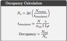
| + | <center><math>t_{simulated}=\frac{N_{events}}{\sigma_{events} \Phi \rho \ell}=\frac{1000000\ barn \cdot s}{7.87\times 10^{-2} \cdot 1.33\times 10^{11}\ barn}=9.54\times 10^{-5} s</math></center> | ||
| + | |||
| + | |||
| + | |||
| + | |||
| + | |||
| + | <center><math>N_0=\Delta t \cdot R_{events}=\Delta t \cdot \frac{N_{events}}{t_{simulated}}=500\times 10^{-9}\ s \cdot \frac{1\times 10^6}{0.0954\times 10^{-3}\ s}=5240</math></center> | ||
| + | |||
| + | |||
| + | <center><math>Occupancy=\frac{N_{hits}}{N_0}=\frac{N_{hits}}{\Delta t \cdot R_{events}}=\frac{t_{simulated}\cdot N_{hits}}{N_{events}\cdot \Delta t}=</math></center> | ||
| + | |||
| + | Similarly, | ||
| + | |||
| + | |||
| + | <center><math>N_{events} =R_{events}\cdot t_{simulated}=\frac{1.05\times 10^{10}events}{s} \cdot 9.54\times 10^{-5} s=1001700\ events</math></center> | ||
| + | |||
| + | |||
| + | <center><math>N_{Moller} =R_{Moller}\cdot t_{simulated}=\frac{9.97\times 10^{9}Moller}{s} \cdot 9.54\times 10^{-5} s=951138\ Moller</math></center> | ||
| + | |||
| + | |||
| + | <center><math>\sigma=\frac{N_{events}}{N_{incident}}\frac{1}{\rho \ell}\Rightarrow N_{incident}=\frac{N_{events}}{\sigma \rho \ell}=\frac{951138}{.075\cdot 2.11\times 10^{-1}}=6\times 10^7\ incident </math></center> | ||
| + | |||
| + | |||
| + | |||
| + | <center><math>\left ( \frac{Number\ of\ hits}{Moller\ electron}\right ) \left (\frac{Moller\ electrons}{incidents\ electron} \right) \left (\frac{incident\ electrons}{sec} \right )</math></center> | ||
Revision as of 20:10, 30 December 2016
Introduction
Moller Scattering
Moller Scattering Definition
Variables_Used_in_Elastic_Scattering
DV_Calculations_of_4-momentum_components
Moller Differential Cross-Section
GEANT4 Simulation of Moller Scattering
LH2 Target
Simulation Setup
NH2 Target
LH2 Vs. NH3
Effects Due to Target Material
Target Density
Atomic Mass and Electron Number Effects
Differential Cross-Section Offset
Weighted Isotropic Distribution in Lab Frame
GEMC Simulation
Drift Chamber
Determining wire-theta correspondence
CED Verification of DC Angle Theta and Wire Correspondance
DC Super Layer 1:Layer 1
DC Binning Based On Wire Numbers
Detector Occupancy
Comparing Rates
Using the values from Whitney:

For a 5cm target of LH2:
Using the beam current of 100nA,
Given the beam Luminosity of:
We can check to make sure the density makes sense
Using the values from Whitney :
https://wiki.iac.isu.edu/index.php/CLAS12_RateEst_byWA
| Energy | 6 GeV | 11 GeV |
| Process | (nb) | (nb) |
| Moller | 22773001 | 75008636 |
| DIS + radiative tail | 128 | 83 |
| Elastic e-p | 5511220 | 3670740 |
| Elastic radiative tail | 24705 | 12944 |
| π0 electro-production | 14802 | 17908 |
| π0 photo-production | 569 | 852 |
| π+ electro-production | 4032 | 5536 |
| π+ photo-production | 282 | 487 |
| π− electro-production | 2806 | 3843 |
| π− photo-production | 199 | 342 |
| Total | 2.83317E7 | 7.87214E7 |


Similarly,