Latest revision as of 02:30, 30 May 2019

Figure 5c: The experimental and theoretical Moller electron differential cross-section for an incident 11 GeV(Lab) electron in the Center of Mass frame of reference.

NH2 Target

Replacing the LH2 target with an NH3 target

Benchmark GEANT4's Moller scattering prediction with the theoretical cross section using NH3

Comparison of simulation vs. the theoretical Møller differential cross section using 11 GeV electrons impinging NH3

Theoretical and Simulated Moller Differential Cross-Section in Center of Mass Frame Frame

Figure 5c: The theoretical and simulated Moller electron differential cross-section for an incident 11 GeV(Lab) electron in the Center of Mass frame of reference for NH3 target.

LH2 Vs. NH3

Benchmark GEANT4's Moller scattering prediction for NH3 and LH2

Effects Due to Target Material

Atomic Mass and Electron Number Effects

Differential Cross-Section Offset

Figure 5c: The theoretical and simulated Moller electron differential cross-section for an incident 11 GeV(Lab) electron in the Center of Mass frame of reference for NH3 target. The theoretical differential cross-section has been adjusted to account for the 10 electrons within NH3.

Modeling the EG12 Drift Chamber

Mathematica Simulation

In the Detector Frame

Preparing Drift Chamber Efficiency Tests

Understanding GEMC Component Effects

rename "s/.stl/.junk/" *.stl

Mlr_Summ_TF

Results

DV_RunGroupC_Moller

Monte Carlo Binary Collision Approximation

@@ Line 3: / Line 3: @@
 =Moller Scattering=
 ==Moller Scattering Definition==
-===[[Variables_Used_in_Elastic_Scattering]]===
+==[[Relativistic Frames of Reference]]==
+===[[Relativistic Units]]===
+==[[4-vectors]]==
-===[[DV_Calculations_of_4-momentum_components]]===
+===[[4-momenta]]===
+===[[Frame of Reference Transformation]]===
+===[[4-gradient]]===
-==[[DV_XSECT|Moller Differential Cross-Section]]==
+==[[Mandelstam Representation]]==
+===[[s-Channel]]===
+===[[t-Channel]]===
+===[[u-Channel]]===
+===[[Limits based on Mandelstam Variables]]===
+====[[Limit of Energy in Lab Frame]]====
+====[[Limit of Scattering Angle Theta in Lab Frame]]====
-=GEANT4 Simulation of Moller Scattering=
+==Initial 4-momentum Components==
-==LH2 Target==
-=== [[LH2 target|Simulation Setup]]===
+===[[Initial Lab Frame 4-momentum components]]===
-==NH2 Target==
+===[[Initial CM Frame 4-momentum components]]===
+===[[Special Case of Equal Mass Particles]]===
+====[[Total Energy in CM Frame]]====
+====[[Scattered and Moller Electron Energies in CM Frame]]====
+==Final 4-momentum components==
+===[[Final Lab Frame Moller Electron 4-momentum components in XZ Plane]]===
+===[[Final Lab Frame Moller Electron 4-momentum components in XY Plane]]===
+====[[Momentum Components in the XY Plane Based on Angle Phi]]====
+===[[Final CM Frame Moller Electron 4-momentum components]]===
+===[[Final CM Frame Scattered Electron 4-momentum components]]===
+===[[Final Lab Frame Scattered Electron 4-momentum components]]===
-==LH2 Vs. NH3==
+==[[Summary of 4-momentum components]]==
-==Effects Due to Target Material==
+==[[Verification of 4-momentum components]]==
-===[[DV_Target_Density|Target Density]]===
+==[[Feynman Calculus]]==
+===[[Flux of Incoming Particles]]===
+===[[Invariant Lorentz Phase Space]]===
-===[[DV_a_z_target|Atomic Mass and Electron Number Effects]]===
+===[[Relativistic Differential Cross-section]]===
-==Differential Cross-Section Offset==
+==[[Scattering Amplitude]]==
-=Weighted Isotropic Distribution in Lab Frame=
+==[[Differential Cross-Section]]==
+==[[DV_XSECT|Moller Differential Cross-Section]]==
+===[[DV_Plotting_XSect | Plotting the Differential Cross-section]]===
-=GEMC Simulation=
+=GEANT4 Simulation of Moller Scattering of Target Material=
+==LH2 Target==
+=== [[LH2 target|6e7 incident electrons on 1cm square LH2 target Simulation Setup]]===
-==Drift Chamber==
+=== [[LH2 target2|6e7 incident electrons on 5cm cylinder LH2 target Simulation Setup]]===
-===[[Determining wire-theta correspondence]]===
-===CED Verification===
+=== [[LH2 target3|6e7 incident electrons on 1mm cylinder LH2 target Simulation Setup]]===
-Using CED to verify the angle and wire correlation,
+====[[Converting to barns|Converting the number of scattered electrons per scattering angle theta to a differential cross-section in barns.]]====
+====[[DV_Moller_LH2 | Benchmark GEANT4's Moller scattering prediction with the theoretical cross section using LH2]]====
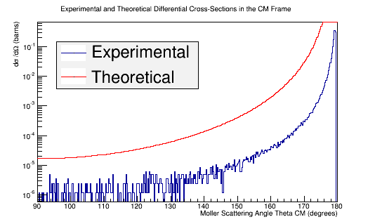
-Zooming in on the view paralell to the direction of the wires in ced, we can examine the wire corresponding theta angle in the drift chamber.
-<center>[[File:ParallelWireZoom.png]]</center>
+===Comparison of simulation vs. the theoretical Møller differential cross section using 11 GeV electrons impinging LH2===
+[[Converting to barns|Converting the number of scattered electrons per scattering angle theta to a differential cross-section in barns.]]
-{|   border=1 align=center
+[[File:XSect_new_zoom.png|frame|center|alt=Experimental and Theoretical Moller Differential Cross-Section in Center of Mass Frame Frame|'''Figure 5c:''' The experimental and theoretical Moller electron differential cross-section for an incident 11 GeV(Lab) electron in the Center of Mass frame of reference.]]
-  |+ Table 1: Superlayer 1 Wire 1 Coordinates
-|- style="font-weight:bold; text-align:center;"
-  !  style=" border:1px solid gray;"|Coordinates(cm)
-  ! style=" border:1px solid gray;"|Layer 1
-  ! style=" border:1px solid gray;"|Layer 2
-  !  style=" border:1px solid gray;"|Layer 3
- ! style=" border:1px solid gray;"|Layer 4
-  ! style=" border:1px solid gray;"|Layer 5
-  ! style=" border:1px solid gray;"|Layer 6
-|-
-  | style="border:1px solid gray;"|'''x'''
-  | style="border:1px solid gray;"|20.42
-  | style="border:1px solid gray;"|21.51
-  | style="border:1px solid gray;"|21.39
- | style="border:1px solid gray;"|22.49
-  | style="border:1px solid gray;"|22.37
-  | style="border:1px solid gray;"|23.47
-|-
-  | style="border:1px solid gray;"|'''y'''
-  | style="border:1px solid gray;"|0.00
-  | style="border:1px solid gray;"|0.00
-  | style="border:1px solid gray;"|0.00
- | style="border:1px solid gray;"|0.00
-  | style="border:1px solid gray;"|0.00
-  | style="border:1px solid gray;"|0.00
-|-
-  | style="border:1px solid gray;"|'''z'''
-  | style="border:1px solid gray;"|243.41
-  | style="border:1px solid gray;"|244.18
-  | style="border:1px solid gray;"|245.51
- | style="border:1px solid gray;"|246.28
-  | style="border:1px solid gray;"|247.62
-  | style="border:1px solid gray;"|248.38
-|}
-{|   border=1 align=center
+===[[Effects Due to Target Length]]===
-  |+ Table 2: Superlayer 1 Wire 2 Coordinates
-|- style="font-weight:bold; text-align:center;"
-  !  style=" border:1px solid gray;"|Coordinates(cm)
-  ! style=" border:1px solid gray;"|Layer 1
-  ! style=" border:1px solid gray;"|Layer 2
-  !  style=" border:1px solid gray;"|Layer 3
- ! style=" border:1px solid gray;"|Layer 4
-  ! style=" border:1px solid gray;"|Layer 5
-  ! style=" border:1px solid gray;"|Layer 6
-|-
-  | style="border:1px solid gray;"|'''x'''
-  | style="border:1px solid gray;"|21.64
-  | style="border:1px solid gray;"|22.73
-  | style="border:1px solid gray;"|22.61
- | style="border:1px solid gray;"|23.71
-  | style="border:1px solid gray;"|23.58
-  | style="border:1px solid gray;"|24.69
-|-
-  | style="border:1px solid gray;"|'''y'''
-  | style="border:1px solid gray;"|0.00
-  | style="border:1px solid gray;"|0.00
-  | style="border:1px solid gray;"|0.00
- | style="border:1px solid gray;"|0.00
-  | style="border:1px solid gray;"|0.00
-  | style="border:1px solid gray;"|0.00
-|-
-  | style="border:1px solid gray;"|'''z'''
-  | style="border:1px solid gray;"|242.86
-  | style="border:1px solid gray;"|243.62
-  | style="border:1px solid gray;"|244.94
- | style="border:1px solid gray;"|245.71
-  | style="border:1px solid gray;"|247.05
-  | style="border:1px solid gray;"|247.81
-|}
-Corresponding theta angles can be found for other wires, in Region 1, Superlayers 1 and 2.
+==NH2 Target==
+===[[Replacing the LH2 target with an NH3 target]]===
+==[[DV_Moller_NH3|Benchmark GEANT4's Moller scattering prediction with the theoretical cross section using NH3]]==
-{|   border=1 align=center
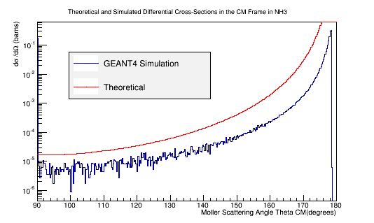
+==Comparison of simulation vs. the theoretical Møller differential cross section using 11 GeV electrons impinging NH3==
-  |+ Table 3: Superlayer 1 Wire-Angle Theta Correspondence in Degrees
-|- style="font-weight:bold; text-align:center;"
-  !  style=" border:1px solid gray;"|Wire Number
-  ! style=" border:1px solid gray;"|Layer 1
-  ! style=" border:1px solid gray;"|Layer 2
-  !  style=" border:1px solid gray;"|Layer 3
- ! style=" border:1px solid gray;"|Layer 4
-  ! style=" border:1px solid gray;"|Layer 5
-  ! style=" border:1px solid gray;"|Layer 6
-|-
-  | style="border:1px solid gray;"|'''1'''
-  | style="border:1px solid gray;"|4.79
-  | style="border:1px solid gray;"|5.03
-  | style="border:1px solid gray;"|4.98
- | style="border:1px solid gray;"|5.22
-  | style="border:1px solid gray;"|5.16
-  | style="border:1px solid gray;"|5.40
-|-
-  | style="border:1px solid gray;"|''' 2'''
-  | style="border:1px solid gray;"|5.09
-  | style="border:1px solid gray;"|5.33
-  | style="border:1px solid gray;"|5.27
- | style="border:1px solid gray;"|5.51
-  | style="border:1px solid gray;"|5.45
-  | style="border:1px solid gray;"|5.69
-|-
-  | style="border:1px solid gray;"|''' 62'''
-  | style="border:1px solid gray;"|24.42
-  | style="border:1px solid gray;"|
-  | style="border:1px solid gray;"|
- | style="border:1px solid gray;"|
-  | style="border:1px solid gray;"|
-  | style="border:1px solid gray;"|
-|-
-  | style="border:1px solid gray;"|''' 63'''
-  | style="border:1px solid gray;"|24.76
-  | style="border:1px solid gray;"|
-  | style="border:1px solid gray;"|
- | style="border:1px solid gray;"|
-  | style="border:1px solid gray;"|
-  | style="border:1px solid gray;"|
-|-
-  | style="border:1px solid gray;"|''' 64'''
-  | style="border:1px solid gray;"|25.10
-  | style="border:1px solid gray;"|
-  | style="border:1px solid gray;"|
- | style="border:1px solid gray;"|
-  | style="border:1px solid gray;"|
-  | style="border:1px solid gray;"|
-|-
-  | style="border:1px solid gray;"|'''77'''
-  | style="border:1px solid gray;"|29.46
-  | style="border:1px solid gray;"|29.60
-  | style="border:1px solid gray;"|29.41
- | style="border:1px solid gray;"|29.55
-  | style="border:1px solid gray;"|29.37
-  | style="border:1px solid gray;"|29.51
-|-
-  | style="border:1px solid gray;"|'''78'''
-  | style="border:1px solid gray;"|29.79
-  | style="border:1px solid gray;"|29.93
-  | style="border:1px solid gray;"|29.74
- | style="border:1px solid gray;"|29.88
-  | style="border:1px solid gray;"|29.69
-  | style="border:1px solid gray;"|29.83
-|-
-  | style="border:1px solid gray;"|'''79'''
-  | style="border:1px solid gray;"|30.12
-  | style="border:1px solid gray;"|30.26
-  | style="border:1px solid gray;"|30.07
- | style="border:1px solid gray;"|30.21
-  | style="border:1px solid gray;"|30.02
-  | style="border:1px solid gray;"|30.16
-|-
-  | style="border:1px solid gray;"|'''110'''
-  | style="border:1px solid gray;"|40.19
-  | style="border:1px solid gray;"|40.28
-  | style="border:1px solid gray;"|40.05
- | style="border:1px solid gray;"|40.13
-  | style="border:1px solid gray;"|39.91
-  | style="border:1px solid gray;"|39.99
-|-
-  | style="border:1px solid gray;"|'''111'''
-  | style="border:1px solid gray;"|40.51
-  | style="border:1px solid gray;"|40.59
-  | style="border:1px solid gray;"|40.36
- | style="border:1px solid gray;"|40.44
-  | style="border:1px solid gray;"|40.21
-  | style="border:1px solid gray;"|40.29
-|-
-  | style="border:1px solid gray;"|''' 112'''
-  | style="border:1px solid gray;"|40.82
-  | style="border:1px solid gray;"|40.90
-  | style="border:1px solid gray;"|40.67
- | style="border:1px solid gray;"|40.75
-  | style="border:1px solid gray;"|40.52
-  | style="border:1px solid gray;"|40.60
-|}
+[[File:XSect_NH3.png|frame|center|alt=Theoretical and Simulated Moller Differential Cross-Section in Center of Mass Frame Frame|'''Figure 5c:''' The theoretical and simulated Moller electron differential cross-section for an incident 11 GeV(Lab) electron in the Center of Mass frame of reference for NH3 target.]]
-{|   border=1 align=center
+==LH2 Vs. NH3==
-  |+ Table 4: Superlayer 2 Wire-Angle Theta Correspondence in Degrees
+===[[DV_Moller_NH3_LH2|Benchmark GEANT4's Moller scattering prediction for NH3 and LH2]]===
-|- style="font-weight:bold; text-align:center;"
-  !  style=" border:1px solid gray;"|Wire Number
-  ! style=" border:1px solid gray;"|Layer 1
-  ! style=" border:1px solid gray;"|Layer 2
-  !  style=" border:1px solid gray;"|Layer 3
- ! style=" border:1px solid gray;"|Layer 4
-  ! style=" border:1px solid gray;"|Layer 5
-  ! style=" border:1px solid gray;"|Layer 6
-|-
-  | style="border:1px solid gray;"|'''1'''
-  | style="border:1px solid gray;"|4.79
-  | style="border:1px solid gray;"|5.03
-  | style="border:1px solid gray;"|4.98
- | style="border:1px solid gray;"|5.22
-  | style="border:1px solid gray;"|5.16
-  | style="border:1px solid gray;"|5.40
-|-
-  | style="border:1px solid gray;"|''' 2'''
-  | style="border:1px solid gray;"|5.09
-  | style="border:1px solid gray;"|5.33
-  | style="border:1px solid gray;"|5.27
- | style="border:1px solid gray;"|5.51
-  | style="border:1px solid gray;"|5.45
-  | style="border:1px solid gray;"|5.69
-|-
-  | style="border:1px solid gray;"|'''77'''
-  | style="border:1px solid gray;"|29.46
-  | style="border:1px solid gray;"|29.60
-  | style="border:1px solid gray;"|29.41
- | style="border:1px solid gray;"|29.56
-  | style="border:1px solid gray;"|29.37
-  | style="border:1px solid gray;"|29.51
-|-
-  | style="border:1px solid gray;"|'''78'''
-  | style="border:1px solid gray;"|29.79
-  | style="border:1px solid gray;"|29.93
-  | style="border:1px solid gray;"|29.74
- | style="border:1px solid gray;"|29.88
-  | style="border:1px solid gray;"|29.70
-  | style="border:1px solid gray;"|29.84
-|-
-  | style="border:1px solid gray;"|'''79'''
-  | style="border:1px solid gray;"|30.13
-  | style="border:1px solid gray;"|30.27
-  | style="border:1px solid gray;"|30.07
- | style="border:1px solid gray;"|30.21
-  | style="border:1px solid gray;"|30.02
-  | style="border:1px solid gray;"|30.16
-|-
-  | style="border:1px solid gray;"|'''110x'''
-  | style="border:1px solid gray;"|40.19
-  | style="border:1px solid gray;"|40.28
-  | style="border:1px solid gray;"|40.05
- | style="border:1px solid gray;"|40.13
-  | style="border:1px solid gray;"|39.91
-  | style="border:1px solid gray;"|39.99
-|-
-  | style="border:1px solid gray;"|'''111'''
-  | style="border:1px solid gray;"|40.51
-  | style="border:1px solid gray;"|40.59
-  | style="border:1px solid gray;"|40.36
- | style="border:1px solid gray;"|40.44
-  | style="border:1px solid gray;"|40.22
-  | style="border:1px solid gray;"|40.30
-|-
-  | style="border:1px solid gray;"|''' 112'''
-  | style="border:1px solid gray;"|40.82
-  | style="border:1px solid gray;"|40.90
-  | style="border:1px solid gray;"|40.67
- | style="border:1px solid gray;"|40.75
-  | style="border:1px solid gray;"|40.52
-  | style="border:1px solid gray;"|40.60
-|}
-====Super Layer 1:Layer 1====
+==Effects Due to Target Material==
-{|   border=1 align=center
+===[[DV_Target_Density|Target Density]]===
-  |+ Table 1: Superlayer 1 Change of Coordinates From Wire 1 to Wire 2(cm)
-|- style="font-weight:bold; text-align:center;"
-  !  style=" border:1px solid gray;"|Coordinates(cm)
-  ! style=" border:1px solid gray;"|Layer 1
-  ! style=" border:1px solid gray;"|Layer 2
-  !  style=" border:1px solid gray;"|Layer 3
- ! style=" border:1px solid gray;"|Layer 4
-  ! style=" border:1px solid gray;"|Layer 5
-  ! style=" border:1px solid gray;"|Layer 6
-|-
-  | style="border:1px solid gray;"|'''<math>\Delta x</math>'''
-  | style="border:1px solid gray;"|1.22
-  | style="border:1px solid gray;"|1.22
-  | style="border:1px solid gray;"|1.22
- | style="border:1px solid gray;"|1.22
-  | style="border:1px solid gray;"|1.21
-  | style="border:1px solid gray;"|1.22
-|-
-  | style="border:1px solid gray;"|'''<math>\Delta y</math>'''
-  | style="border:1px solid gray;"|0.00
-  | style="border:1px solid gray;"|0.00
-  | style="border:1px solid gray;"|0.00
- | style="border:1px solid gray;"|0.00
-  | style="border:1px solid gray;"|0.00
-  | style="border:1px solid gray;"|0.00
-|-
-  | style="border:1px solid gray;"|'''<math>\Delta z</math>'''
-  | style="border:1px solid gray;"|.55
-  | style="border:1px solid gray;"|.56
-  | style="border:1px solid gray;"|.57
- | style="border:1px solid gray;"|.57
-  | style="border:1px solid gray;"|.57
-  | style="border:1px solid gray;"|.57
-|}
-Using the geometric construction for determining angle theta to wire 2:
+===[[DV_a_z_target|Atomic Mass and Electron Number Effects]]===
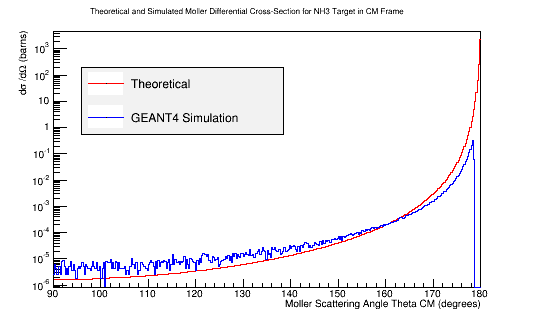
-<center><math>\tan{\theta}=\frac{x+\Delta x}{z+\Delta z}\Rightarrow \theta=\arctan{\frac{x+\Delta x}{z+\Delta z}}</math></center>
+==[[Calculating the differential cross-sections for the different materials, and placing them as well as the theoretical differential cross-section into a plot:|Differential Cross-Section Offset]]==
-<center><math>\arctan{\frac{20.42+1.212}{243.39-0.5652}}=\arctan{\frac{21.632}{242.8248}}=\arctan{0.0891}=5.09^{\circ}</math></center>
+[[File:Adjusted_MollerXSect_NH3.png‎|frame|center|alt=Theoretical and Simulated Moller Differential Cross-Section in Center of Mass Frame Frame|'''Figure 5c:''' The theoretical and simulated Moller electron differential cross-section for an incident 11 GeV(Lab) electron in the Center of Mass frame of reference for NH3 target.  The theoretical differential cross-section has been adjusted to account for the 10 electrons within NH3.]]
+=Modeling the EG12 Drift Chamber=
-This equation can be solved for a hypothetical wire 0, which will allow the wire number to be the multiplicative factor for the change from the starting position.
+==Drift Chamber==
+===[[Determining wire-theta correspondence]]===
+====[[GEMC Verification]]====
-<center><math>\tan{\theta}=\frac{x-\Delta x+n\Delta x}{z-\Delta z+n\Delta z}\Rightarrow \theta=\arctan{\frac{x'+n\Delta x}{z'+n\Delta z}}</math></center>
+====[[CED Verification of DC Angle Theta and Wire Correspondance]]====
-where
+====[[DC Super Layer 1:Layer 1]]====
-<center><math>x'=20.42-1.212\approx 19.21cm</math></center>
+===[[DC Binning Based On Wire Numbers]]===
-<center><math>z'=243.39+0.5652\approx 243.96cm</math></center>
-<center><math>\theta=\arctan{\frac{19.21+n1.212}{243.39-n0.5652}}</math></center>
+===[[Detector_Geometry Simulation]]===
+====[[Conic Sections]]====
+=====[[Circular Cross Sections]]=====
+=====[[Elliptical Cross Sections]]=====
-<center><math>\tan{\theta}=\frac{19.21+n1.212}{243.39-n0.5652}\Rightarrow \tan{ \theta}=-2.14437 + \frac{957.412}{430.626 - n}\Rightarrow 430.626 - n = \frac{957.412}{\tan{ \theta}+2.14437}</math></center>
+====[[Determing Elliptical Components]]====
+====[[Determing Elliptical Equations]]====
+=====[[Test for Theta at 20 degrees and Phi at 0]]=====
+====[[In the Detector Plane]]====
+=====[[Test in Plane for Theta at 20 degrees and Phi at 0]]=====
+=====[[Test in Plane for Theta at 20 degrees and Phi at 1 degree]]=====
+===[[Function for change in x', Lab frame]]===
+===[[Wire Number Function]]===
+===Mathematica Simulation===
+====[[In the Detector Frame]]====
-<center><math>\Rightarrow n = \frac{-957.412}{\tan{ \theta}+2.14437}+430.626</math></center>
+====In the wire frame====
+=====[[Points of Intersection]]=====
+=====[[The Wires]]=====
+=====[[Right Hand Wall]]=====
+=====[[Left Hand Wall]]=====
+=====[[The Ellipse]]=====
+====[[Plotting Different Frames]]====
+====[[Parameterizing the Ellipse Equation]]====
+====[[Change in Wire Bin Number]]====
+===One Hit per Wire Bin===
-Using Mathematica, a series expansion about n=0 can be found:
+====[[One Hit Per Wire Bin|One Hit Per Wire Bin at phi=0]]====
-<pre>
+====[[Wire Bin Number as a function of Theta and Phi for Right Side]]====
-In[1]:= Series[ArcTan[(19.21+1.212 x)/(243.39-0.5652 n)],{n,0,4}]
-Out[1]= 0.0787635+0.00513098 n+9.83726*10^-6 n^2-2.61675*10^-8 n^3-2.22826*10^-10 n^4+O[n]^5
+====[[Wire Bin Number as a function of Theta and Phi for Left Side]]====
-</pre>
-<center><math>\theta\approx 0.0787635+0.00513098 n+9.83726\times 10^{-6} n^2-2.61675\times 10^{-8} n^3</math></center>
+=[[Preparing Drift Chamber Efficiency Tests]]=
+==[[Uniform distribution in Energy and Theta LUND files]]==
-This expression will find the angle theta in radians given the wire number.  To convert from radians to degrees, we can multiply by 180 and divide by Pi.
+===[[1000 Events per degree in the range 5 to 40 degrees for Lab Frame]]===
+===[[Isotropic Spread in CM for 5 to 40 degrees in Lab Frame|Isotropic Spread in CM for 5 to 40 degrees in Lab Frame at Phi=0]]===
+===[[Isotropic Spread  in Lab Frame for 5 to 40 degrees in Theta and for Phi between -30 and 30 Degrees]]===
-<pre>
+===[[Reading_LUND_files]]===
-In[2]:= 180*(0.07876354504106763`+0.005130982891104289` n+9.837257652182922`*^-6 n^2-2.616751708660921`*^-8 n^3-2.2282595631625944`*^-10 n^4+O[n]^5)/3.14159625359
+===[[Run GEMC Isotropic Theta and Phi for Sector 1 DC]]===
-Out[2]= 4.51281+0.293983 n+0.000563633 n^2-1.49929*10^-6 n^3-1.2767*10^-8 n^4+O[n]^5
+===[[Analysis of evio files]]===
-</pre>
+====[[Little Runs]]====
+====[[Bin Test]]====
+====[[Field Test]]====
+====[[Bin Shapes]]====
+====[[Limit Adjustment on Walls]]====
+===[[HITs in DC]]===
+===[[Hits with Changing Torus Field and 0T Solenoid]]===
+====[[Too Large Events]]====
-<center><math>\theta\approx 4.51281+0.293983 n+0.000563633 n^2-1.49929\times10^{-6} n^3</math></center>
+===[[Hits with -5T Torus and Changing Solenoid Field]]===
+===[[Weight]]===
+==Detector Occupancy==
+===[[Defining Occupancy]]===
+====[[Unweighted Occupancy]]====
+====[[Weighted Occupancy]]====
+====[[Rates]]====
+=====[[Gamma Event Vertex]]=====
-This tells us that the expression for theta will follow a function that comes from a series expansion.  To account for instrument and measurement errors, angle measurements from ced can be used to find a better fit.
+===[[Comparing With Whitney Rates|Whitney Rates]]===
-Using Mathematica, a line can be fitted to the data collected on the wire number to angle theta correspondence.
-Declaring the data set:
-<pre>
-In[1]:= data1={{1,4.79},{2,5.09},{62,24.42},{63,24.76},{64,25.10},{78,29.79},{111,40.50},{112,40.82}}
-Out[1]= {{1,4.79},{2,5.09},{62,24.42},{63,24.76},{64,25.1},{78,29.79},{111,40.5},{112,40.82}}
-</pre>
-Testing for a linear fit:
-<pre>
-In[2]:= line1=Fit[data1,{1,n},n]
-Out[2]= 4.39975 + 0.32469 n
-</pre>
-Examing the range limits for the angle theta for layer 1:
-Taking the difference of the upper and lower limits in theta,
-<center><math>\Delta degrees=40.82^{\circ}-4.79^{\circ}=36.03^{\circ}</math></center>
-Dividing by the change in wire numbers (112-1=111), we find
-<center><math>\frac{\Delta degrees}{\Delta wire\ number}=\frac{36.03^{\circ}}{111\ wires}\approx\  \frac{0.325^{\circ}}{wire\ number}</math></center>
-This would imply that if the wires were evenly placed, their change in angle theta would increase by the factor of .325 degrees for each increase in wire number, starting obviously with wire 1 at 4.79 degrees.  In addition, this implies that the bin spacing for each wire would be around .325 degrees in width.
+===[[GEANT Moller Simulations Comparison|GEANT Moller Simulations]]===
+===[[Comparison of GEANT Simulation to Whitney Data]]===
+===[[Occupancy for Sector 1]]===
-Chercking this, we can find the difference between wires 1 and 2,
+===[[Rates for Sector 1]]===
+===[[Rates for Different Currents]]===
+====[[Rates for Different Solenoid Strengths]]====
+====[[Rates for all Sectors based on Initial Sector 1 incident Moller electrons]]====
+====[[Changing Solenoid Field Rates in Sector 1]]====
+====[[Pb Cylinder (AKA "Temp Shield")]]====
-<center><math>\frac{\Delta degree}{\Delta wire\ number}=\frac{5.09^{\circ}-4.79^{\circ} }{wire\ number}=\frac{.3^{\circ}}{wire\ number} </math></center>
+=[[Understanding GEMC Component Effects]]=
+<pre>rename "s/.stl/.junk/" *.stl</pre>
+==[[Forward Chamber]]==
+==[[Drift Chamber]]==
+==[[Magnets]]==
+===[[Solenoid]]===
+===[[Torus]]===
+===[[CAD Components]]===
+====[[BoreShield]]====
+====[[CenterTube]]====
+====[[DownstreamShieldingPlate]]====
+====[[DownstreamVacuumJacket]]====
+====[[Hub001]]====
+====[[Plates 1-6]]====
+====[[Shields 1-7]]====
-Similarly, finding the difference between wires 111 and 112,
+====[[UpstreamShieldingPlate]]====
+====[[UpstreamVacuumJacket]]====
+====[[WarmBoreTube]]====
+====[[coils 1-6]]====
+====[[shell 1-6 a/b]]====
+====[[dc supports sectors 1-6 region 1]]====
+====[[dc back sectors 1-6 region 1]]====
+====[[apex]]====
+==[[Beamline]]==
+===[[CadBeamline]]===
+====[[innerShieldAndFlange]]====
+====[[outerFlange]]====
+====[[outerMount]]====
+====[[nut 1-9]]====
+====[[taggerInnerShield]]====
+====[[main-cone]]====
+====[[adjuster 1-3]]====
+====[[DSShieldFrontLead]]====
+====[[DSShieldBackLead]]====
+====[[DSShieldInnerAss]]====
+====[[DSShieldBackAss]]====
+====[[DSShieldFrontAss]]====
+====[[DSShieldBackCover]]====
+====[[DSShieldFrontCover]]====
+====[[DSShieldFlangeAttachment]]====
+====[[DSShieldFlange]]====
+===[[VacuumLine]]===
+====[[ConnectUpstreamToTorusPipe]]====
+====[[connectTorusToDownstreamPipe]]====
+====[[downstreamPipeFlange]]====
-<center><math>\frac{\Delta degree}{\Delta wire\ number}=\frac{40.82^{\circ}-40.51^{\circ}}{wire\ number}=\frac{.31^{\circ}}{wire\ number}</math></center>
+=[[Mlr_Summ_TF]]=
-These differing values show that the bin width is not uniform in length, therefore a first order, linear fit, will not suffice.
+=[[Results]]=
+[[DV_RunGroupC_Moller]]
+=[[Monte Carlo Binary Collision Approximation]]=
-Testing for a quadratic fit:
-<pre>
-In[3]:= quad1=Fit[data1,{1,n,n^2},n]
-Out[3]= 4.45564 +0.32015 n+0.0000417787 n^2
-</pre>
-The quadratic fit does not work since it's first derivative
-<center><math>\theta'\approx \Delta \theta=.325072-6.83308\ n</math></center>
-does not give the same spacing between low and high values of n as seen in the ced data.  The coefficient near the first order will have to smaller than .31 to find a correlation that would agree.
-Testing for a polynomial of degree 3 fit:
-<pre>
-In[4]:= polynomial1=Fit[data1,{1,n,n^2,n^3},n]
-Out[4]= 4.49876 +0.293001 n+0.000679074 n^2-3.57132*10^-6 n^3
-</pre>
-This fit best matches the data found in ced
-<center><math>\theta\equiv 4.49876 +0.293001 n+0.000679074 n^2-3.57132\times 10^{-6} n^3</math></center>
-As discussed earlier, taking the 1st derivative of this function will give us the spacing of the bins as a function of wire number.
-<center><math>\theta '\equiv 0.293001 + 0.00135815 n - 0.000010714 n^2</math></center>
-The derivative of this function then will tell us where the bin spacing is at a minimum and a maximum.
-<center><math>\theta ''\equiv .001021976-1.61514\times 10^{-5} n</math></center>
-<center><math>0.00135815 - 0.0000214279 n=0\Rightarrow Bin\ Spacing\ Maximum\ at\ n=63.3822</math></center>
-Comparing this maximum, we can see from Table 3 that near the maximum of 63 are seperated by larger distances than at n=1 or n=112.  This is the midpoint of the plane as seen in the geometry file.
-====Binning based on wire numbers====
-The bin size based on wire number will need to be a uniform width of 1, as in an increment of 1 between the integer values of the wires.  This uniformity in bin size based on wire numbers is not uniform when viewed by the angle theta due to the Drift Chamber geometry discussed earlier.
-Modifying evioreader
-<center>[[File:Layer1bins.png]]</center>
-<center>[[File:Layer1bins_Isotropic.png]]</center>
-<pre>
-gStyle->SetStripDecimals(kTRUE);
-TF1 *fit_function=new TF1("fit_function","[0]+[1]*x+[2]*x*x+[3]*x*x*x",4.49876,41.12592);
-fit_function->SetParameters(4.49876,0.293001,0.000679074,-0.00000357132);
-TGaxis *A1 = new TGaxis(0,5000,113,5000,"fit_function",510,"-");
-A1->SetTitle("Angle Theta(degrees)");
-A1->Draw();
-</pre>
-<center>[[File:Layer1binWeighted.png]][[File:MolThetaLabWeighted.png]]</center>
-<center>[[File:Layer1binWeighted_Isotropic.png]][[File:MolThetaLabWeighted2.png]]</center>
-Using the expression for n in terms of Theta:
-<center><math>n = \frac{-957.412}{\tan{ \theta}+2.14437}+430.626</math></center>
-This relationship can be used to multiply each Moller Scattering angle theta in the lab frame, with it's differential cross-section weight, to find the Moller differential cross-section as a function of wire number in the lab frame.
-<center>[[File:MolThetaWireWeighted.png]][[File:MolThetaWireWeightedIsotropic.png]]</center>
-<center>[[File:MolThetaWireWeightedAdjusted.png]][[File:MolThetaWireWeightedAdjustedIsotropic.png]]</center>
-<center>[[File:TheoryDCbinsWire.png]][[File:TheoryDCbinsWireIsotropic.png]]</center>
-==Detector Occupancy==

Difference between revisions of "VanWasshenova Thesis"

Latest revision as of 02:30, 30 May 2019

Introduction

Moller Scattering

Moller Scattering Definition

Initial 4-momentum Components

Final 4-momentum components

GEANT4 Simulation of Moller Scattering of Target Material

LH2 Target

Comparison of simulation vs. the theoretical Møller differential cross section using 11 GeV electrons impinging LH2

NH2 Target

Comparison of simulation vs. the theoretical Møller differential cross section using 11 GeV electrons impinging NH3

LH2 Vs. NH3

Effects Due to Target Material

Modeling the EG12 Drift Chamber

Drift Chamber

Mathematica Simulation

In the wire frame

One Hit per Wire Bin

Detector Occupancy