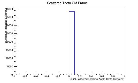
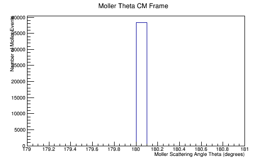
The LUND file is created by creating an isotropic distribution of particles within the Moller Center of Mass frame of reference. These particles are also uniformly distributed through the angle theta with respect to the beam line in the range 90-180 in the Center of Mass frame. This is done at a set angle phi (10 degrees) with respect to the perpendicular components with respect to the beam line.
Center of Mass for Stationary Target
For an incoming electron of 11GeV striking a stationary electron we would expect:
[math]\Longrightarrow \left( \begin{matrix} E^*_{2} \\ p^*_{2(x)} \\ p^*_{2(y)} \\ p^*_{2(z)}\end{matrix} \right)=\left(\begin{matrix}\gamma^* & 0 & 0 & -\beta^* \gamma^*\\0 & 1 & 0 & 0 \\ 0 & 0 & 1 &0 \\ -\beta^* \gamma^* & 0 & 0 & \gamma^* \end{matrix} \right) . \left( \begin{matrix}m\\ 0 \\ 0 \\ 0\end{matrix} \right)[/math]
Phase space Limiting Particles
Since the angle phi has been constrained to remain constant, the x and y components of the momentum will increase in the positive first quadrant. This implies that the z component of the momentum must decrease by the relation:
[math]p^2=p_x^2+p_y^2+p_z^2[/math]
In the Center of Mass frame, this becomes:
[math]p_x^{*2}+p_y^{*2} = p^{*2}-p_z^{*2}[/math]
Since the momentum in the CM frame is a constant, this implies that pz must decrease. For phi=10 degrees:
This is repeated for rotations of 60 degrees in phi in the Lab frame.
We can use the variable rapidity:
[math]y \equiv \frac {1}{2} \ln \left(\frac{E+p_z}{E-p_z}\right)[/math]
where
[math] P^+ \equiv E+p_z[/math]
[math] P^- \equiv E-p_z[/math]
this implies that as
[math]p_z \rightarrow 0 \Rrightarrow \frac{E+p_z}{E-p_z} \rightarrow 1 \Rrightarrow \ln 1 \rightarrow 0 \Rrightarrow y=0[/math]
For forward travel in the light cone:
[math]p_z \rightarrow E \Rrightarrow \frac{E+p_z}{E-p_z} \rightarrow \infin \Rrightarrow \ln \infin \rightarrow \infin \Rrightarrow y \rightarrow \infin [/math]
For backward travel in the light cone:
[math]p_z \rightarrow -E \Rrightarrow \frac{E+p_z}{E-p_z} \rightarrow 0 \Rrightarrow \ln 0 \rightarrow -\infin \Rrightarrow y \rightarrow -\infin [/math]
For a particle that transforms from the Lab frame to the CM frame where the particle is not within the light cone:
[math]p_x^2+p_y^2=52.589054^2+9.272868^2=53.400MeV \gt 53.015 MeV (E) \therefore p_z \rightarrow imaginary[/math]
These particles are outside the light cone and are more timelike, thus not visible in normal space. This will reduce the number of particles that will be detected.
Determining Momentum Components After Collision in CM Frame
The energy and total momentum of the Moller and scattered electron remain the same under a rotation in any frame of reference. After the collision, these quantities remain the same, but the x, y, z components change.
In this frame, we can cycle through values of theta from 90 to 180 degrees which physically correspond to a stationary electron being impinged by an electron.
Theta Dependent Components
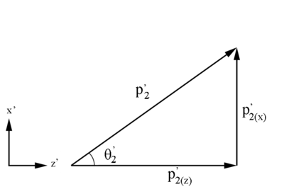 Figure 3: Definition of Moller electron variables in the CM Frame in the x-z plane.
Using [math]\theta '_2=\arccos \left(\frac{p^'_{2(z)}}{p^'_{2}}\right)[/math]
Figure 3: Definition of Moller electron variables in the CM Frame in the x-z plane.
Using [math]\theta '_2=\arccos \left(\frac{p^'_{2(z)}}{p^'_{2}}\right)[/math]
| [math]\Longrightarrow {p^'_{2(z)}=p^'_{2}\cos(\theta '_2)}[/math]
|
Checking on the sign resulting from the cosine function, we are limited to:
| [math]90^\circ \le \theta '_2 \le 180^\circ \equiv \frac{\pi}{2} \le \theta '_2 \le \pi Radians[/math]
|
Since,
[math]\frac{p^'_{2(z)}}{p^'_{2}}=cos(\theta '_2)[/math]
[math]\Longrightarrow p^'_{2(z)}\ should\ always\ be\ negative[/math]
Phi Dependent Components
Since only the z direction is considered to be the relativistic direction of motion, this implies that the x and y components are not effected by a Lorentz transformation and remain the same in the CM and Lab frame. Holding the angle Phi constant at an initial value of 10 degrees, allows us to find the x and y components.
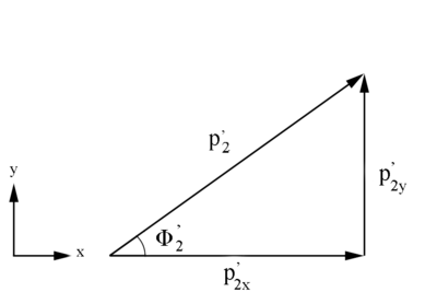 Figure 4: Definition of Moller electron variables in the Lab Frame in the x-y plane.
Similarly, [math]\phi '_2=\arccos \left( \frac{p^'_{2(x) Lab}}{p^'_{2(xy)}} \right)[/math]
Figure 4: Definition of Moller electron variables in the Lab Frame in the x-y plane.
Similarly, [math]\phi '_2=\arccos \left( \frac{p^'_{2(x) Lab}}{p^'_{2(xy)}} \right)[/math]
where [math]p_{2(xy)}^'=\sqrt{(p_{2(x)}^')^2+(p^'_{2(y)})^2}[/math]
[math](p^'_{2(xy)})^2=(p^'_{2(x)})^2+(p^'_{2(y)})^2[/math]
and using [math]p^2=p_{(x)}^2+p_{(y)}^2+p_{(z)}^2[/math]
this gives [math](p^'_{2})^2=(p^'_{2(xy)})^2+(p^'_{2(z)})^2[/math]
[math]\Longrightarrow (p'_{2})^2-(p'_{2(z)})^2 = (p'_{2(xy)})^2[/math]
[math]\Longrightarrow p_{2(xy)}^'=\sqrt{(p^'_{2})^2-(p^'_{2(z)})^2}[/math]
which gives[math]\phi '_2 = \arccos \left( \frac{p_{2(x)}'}{\sqrt{p_{2}^{'\ 2}-p_{2(z)}^{'\ 2}}}\right)[/math]
| [math]\Longrightarrow p_{2(x)}'=\sqrt{p_{2}^{'\ 2}-p_{2(z)}^{'\ 2}} \cos(\phi)[/math]
|
Similarly, using [math]p_{2}^2=p_{2(x)}^2+p_{2(y)}^2+p_{2(z)}^2[/math]
[math]\Longrightarrow p_{2}^{'\ 2}-p_{2(x)}^{'\ 2}-p_{2(z)}^{'\ 2}=p_{2(y)}^{'\ 2}[/math]
| [math]p_{2(y)}'=\sqrt{p_{2}^{'\ 2}-p_{2(x)}^{'\ 2}-p_{2(z)}^{'\ 2}}[/math]
|
Checking on the sign from the cosine results for [math]\phi '_2[/math]
We have the limiting range that [math]\phi[/math] must fall within:
| [math]-\pi \le \phi '_2 \le \pi\ Radians[/math]
|
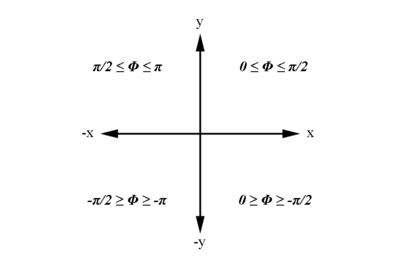
Examining the signs of the components which make up the angle [math]\phi[/math] in the 4 quadrants which make up the xy plane:
| [math]For\ 0 \ge \phi '_2 \ge \frac{-\pi}{2}\ Radians[/math]
|
| px=POSITIVE
|
| py=NEGATIVE
|
| [math]For\ 0 \le \phi '_2 \le \frac{\pi}{2}\ Radians[/math]
|
| px=POSITIVE
|
| py=POSITIVE
|
| [math]For\ \frac{-\pi}{2} \ge \phi '_2 \ge -\pi\ Radians[/math]
|
| px=NEGATIVE
|
| py=NEGATIVE
|
| [math]For\ \frac{\pi}{2} \le \phi '_2 \le \pi\ Radians[/math]
|
| px=NEGATIVE
|
| py=POSITIVE
|
Electron Center of Mass Frame
Relativistically, the x, y, and z components have the same magnitude, but opposite direction, in the conversion from the Moller electron's Center of Mass frame to the electron's Center of Mass frame.
| [math]p^*_{2(x)}= -p^*_{1(x)}[/math]
|
| [math]p^*_{2(y)}= -p^*_{1(y)}[/math]
|
| [math]p^*_{2(z)}=-p^*_{1(z)}[/math]
|
where previously it was shown
| [math]|p^*_{1}|\equiv |p^*_{2}|[/math]
|
| [math]E^*_{1}\equiv E^*_{2}[/math]
|
| [math]\theta_{1}^*=\pi-\theta_{1}^*[/math]
|
Lorentz Transformation to Lab Frame
[math]
\begin{bmatrix}
E_{Lab} \\
P_{x(Lab)} \\
P_{y(Lab)} \\
P_{z(Lab)}
\end{bmatrix}=
\begin{bmatrix}
\gamma & 0 & 0 & \gamma \beta \\
0 & 1 & 0 & 0 \\
0 & 0 & 1 & 0 \\
\gamma \beta & 0 & 0 & \gamma
\end{bmatrix}
\cdot
\begin{bmatrix}
E_{CM} \\
P_{x(CM)} \\
P_{y(CM)} \\
P_{z(CM)}
\end{bmatrix}
[/math]
Weight
Using the theoretical differential cross section from previous
[math]\frac{d\sigma}{d\Omega}=\frac{ \alpha^2 }{4E^2}\frac{ (3+cos^2\theta)^2}{sin^4\theta}[/math]
[math]\alpha ^2=5.3279\times 10^{-5}[/math]
[math]E\approx 53.013 MeV[/math]
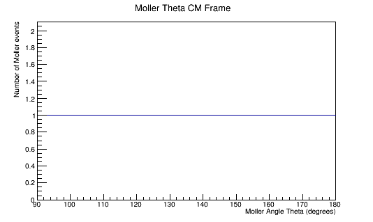
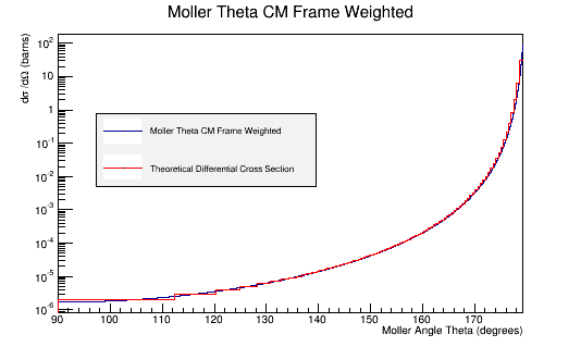
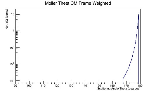
We can take the Moller electron distribution of Theta in the Center of Mass frame, and multiply each given angle Theta by the expected differential cross section.
This causes the Moller Theta distribution in the Center of Mass frame to directly follow the theoretical differential cross section.
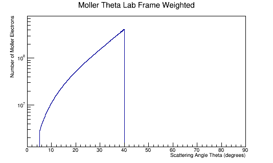
The Lab frame distribution of Theta can also be weighted similarly. However, instead of having it be a differential cross section, we can find the necessary number of particles.
[math]\frac{d\sigma}{d\Omega} = \frac{\left(\frac{number\ of\ particles\ scattered/second}{d\Omega}\right)}{\left(\frac{number\ of\ incoming\ particles/second}{cm^2}\right)}=\frac{dN}{\mathcal L\, d\Omega} =differential\ scattering\ cross\ section[/math]
In order to compute a luminosity for fixed target experiment, it is necessary to take into account the properties of the incoming beam and the stationary target.
[math]\mathcal L = \Phi \rho \ell[/math]
where
[math]\Phi \equiv [/math]flux, or incoming particles per second
[math]\rho \equiv [/math]target density
[math]\ell \equiv [/math]length of target
[math]\frac{d\sigma}{d\Omega} =\frac{dN}{\mathcal L\, d\Omega} =\frac{dN}{\Phi \rho \ell\, d\Omega}[/math]
[math]\Rightarrow \int \frac{d\sigma}{d\Omega} \rho\ \ell \Phi d\Omega=\int dN[/math]
Checking versus the given Luminosity for the experiment
[math]\mathcal L = \frac{1.3 \times 10^{35}}{cm^2\cdot s} \times \frac{10^{-24} cm^2}{barn}=1.35\times 10^{11} barns^{-1}s^{-1}[/math]
[math]\mathcal L \int \frac{d\sigma}{d\Omega} d\Omega = 1.35 \times 10^{11} barns^{-1} \times 2\pi\ \int \frac{d\sigma}{d\Omega}\ \sin{\theta} d\theta=N[/math]
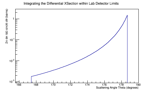
IntegralDiffXSect->Integral()
9.94987649031274486e+03 barns
Multiplying by the Luminosity, we find:
[math]9.95\times 10^{3} barns \times\frac{1.35\times 10^{11}}{barns\cdot s}=1.34\times 10^{15}\frac{electrons}{s}[/math]
Links
Back


