Difference between revisions of "Tamar AnalysisChapt"
| Line 65: | Line 65: | ||
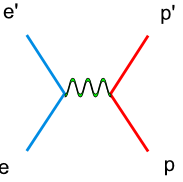
| − | In double spin asymmetry analysis the electron nucleon scattering process is given as an one photon exchange event, so called the Born approximation. In reality, there are multiple photon effects during the experiments. These high order processes, also called radiative effects, can be calculated and used to correct the cross section data. | + | In double spin asymmetry analysis the electron nucleon scattering process is given as an one photon exchange event, so called the Born approximation([https://wiki.iac.isu.edu/images/f/f2/TheBornApproximation.png Fig 1.1.1]). In reality, there are multiple photon effects during the experiments. These high order processes, also called radiative effects, can be calculated and used to correct the cross section data. |
{| border="0" style="background:transparent;" align="center" | {| border="0" style="background:transparent;" align="center" | ||
| Line 74: | Line 74: | ||
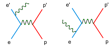
| − | There are two types of radiative corrections, internal and external. Internal radiative corrections describe the contributions which took place during the lepton-hadron interaction. In first order approximation they include vertex photon exchange, self energy and vacuum polarization.<ref name="RadiativeCorrections"> Nucleon Form Factors. In Scholarpedia, from http://www.scholarpedia.org/article/Nucleon_Form_factors#History </ref> | + | There are two types of radiative corrections, internal and external. Internal radiative corrections describe the contributions, which took place during the lepton-hadron interaction. In first order approximation they include vertex photon exchange, self energy and vacuum polarization Fig. 1.1.2 .<ref name="RadiativeCorrections"> Nucleon Form Factors. In Scholarpedia, from http://www.scholarpedia.org/article/Nucleon_Form_factors#History </ref><br> |
| − | |||
{| border="2" align="center" | {| border="2" align="center" | ||
|- | |- | ||
| Line 82: | Line 81: | ||
|[[File:InetranRadiativeCor3.png|350px|thumb|Self Energy]]|| [[File:InetranRadiativeCor4.png|350px|thumb|Self Energy]] | |[[File:InetranRadiativeCor3.png|350px|thumb|Self Energy]]|| [[File:InetranRadiativeCor4.png|350px|thumb|Self Energy]] | ||
|}<br> | |}<br> | ||
| − | + | {| border="2" align="center" | |
| − | + | |- | |
| − | On the other hand, the external radiative corrections account for the Bremsstrahlung by the incoming and scattered electron and by the recoiling target nucleon. | + | |'''Figure 1.1.2''' Internal Radiation |
| + | |}<br> | ||
| + | On the other hand, the external radiative corrections account for the Bremsstrahlung by the incoming and scattered electron and by the recoiling target nucleon [https://wiki.iac.isu.edu/images/0/04/ExternalRadiativeCor.png Fig. 1.1.3].<br> | ||
{| border="0" style="background:transparent;" align="center" | {| border="0" style="background:transparent;" align="center" | ||
|- | |- | ||
| | | | ||
| − | [[File:ExternalRadiativeCor.png|350px|thumb|Externall Radiation]] | + | [[File:ExternalRadiativeCor.png|350px|thumb|'''Figure 1.1.3''' Externall Radiation]] |
|}<br> | |}<br> | ||
| − | + | One of the major advantages of the double polarization experiments is the minimum contribution from the radiative corrections. For the <math>~4.2 GeV</math> incident electron beam data the radiative corrections are less than 5%<ref>http://www.jlab.org/Hall-B/secure/eg1/EG2000/fersch/QUALITY_CHECKS/file_quality/runinfo.txt</ref>. Due to negligible contributions from the radiative corrections, they are not included in the double spin asymmetry analysis.<br> | |
| − | |||
| − | One of the major advantages of the double polarization experiments is the minimum contribution from the radiative corrections. For the ~4.2 GeV incident electron beam data the radiative corrections are less than 5%<ref>http://www.jlab.org/Hall-B/secure/eg1/EG2000/fersch/QUALITY_CHECKS/file_quality/runinfo.txt</ref>. Due to negligible contributions from the radiative corrections they are not included in the double spin asymmetry analysis. | ||
=electron identification= | =electron identification= | ||
Revision as of 17:56, 18 April 2012
Data Analysis
In this chapter, we discuss the techniques used to analyze the data collected during the EG1b experiment and calculate semi-inclusive cross sections for the following reactions: and for NH3 and ND3 polarized targets respectively. The goal of this work is measure the fragmentation function depends on the Bjorken scaling variable () and the four momentum transfer squared () as well as evaluate the independence of the fractional energy of the observed final state hadron (). The fragmentation function ( ) can be expressed in terms of the ratio of the difference of polarized to unpolarized cross sections for the semi inclusive deep inelastic scattering for proton and neutron targets.
There are couple of main steps in the data analysis, which will be discussed bellow in this chapter:
- Electron Identification
- EC cuts
- Cerenkov cuts
- Fidcucial Cuts
- Pion Identification
- Specific Event Reconstruction Efficiency(Inclusive, semi-inclusive and exclusive)
- Beam Charge Asymmetry
- Semi-inclusive Deep Inelastic Scattering Asymmetry(SIDIS)
- and binning
- Statistical and Systematic Errors
- Radiative Corrections
- The ratio of the difference of polarized to unpolarized cross sections for the semi inclusive deep inelastic scattering for proton and neutron
- Models
- Data Selection
The CLAS Data Selection
The data files from the EG1b run were chosen for this analysis. During the experiment, 2.2 GeV, 4.2 GeV and 5.7 GeV longitudinally polarized electron beams were used on the polarized frozen ammonia NH3 and ND3 targets. This work will discuss the analysis of 4.2 GeV electron beam on hydrogen and deuteron targets. The collected data has been filtered by applying restrictions, which will be discussed in tin this chapter below. For the final results, the run sets were combined for each target type.
| Run Set | Target Type | Torus Current(A) | Target Polarization | Half Wave Plane(HWP) |
| 28100 - 28102 | ND3 | +2250 | -0.18 | +1 |
| 28106 - 28115 | ND3 | +2250 | -0.18 | -1 |
| 28145 - 28158 | ND3 | +2250 | -0.20 | +1 |
| 28166 - 28190 | ND3 | +2250 | +0.30 | +1 |
| 28205 - 28217 | NH3 | +2250 | +0.75 | +1 |
| 28222 - 28236 | NH3 | +2250 | -0.68 | +1 |
| 28242 - 28256 | NH3 | +2250 | -0.70 | -1 |
| 28260 - 28275 | NH3 | +2250 | +0.69 | -1 |
| 28287 - 28302 | ND3 | -2250 | +0.28 | +1 |
| 28306 - 28322 | ND3 | -2250 | -0.12 | +1 |
| 28375 - 28399 | ND3 | -2250 | +0.25 | -1 |
| 28407 - 28417 | NH3 | -2250 | +0.73 | -1 |
| 28456 - 28479 | NH3 | -2250 | -0.69 | +1 |
Table 1.1. EG1b Runs used for Analysis.(Run Sets, Target Type, Torus Current, Target Polarization, HWP)
Radiative Corrections
In double spin asymmetry analysis the electron nucleon scattering process is given as an one photon exchange event, so called the Born approximation(Fig 1.1.1). In reality, there are multiple photon effects during the experiments. These high order processes, also called radiative effects, can be calculated and used to correct the cross section data.

There are two types of radiative corrections, internal and external. Internal radiative corrections describe the contributions, which took place during the lepton-hadron interaction. In first order approximation they include vertex photon exchange, self energy and vacuum polarization Fig. 1.1.2 .<ref name="RadiativeCorrections"> Nucleon Form Factors. In Scholarpedia, from http://www.scholarpedia.org/article/Nucleon_Form_factors#History </ref>


| Figure 1.1.2 Internal Radiation |
On the other hand, the external radiative corrections account for the Bremsstrahlung by the incoming and scattered electron and by the recoiling target nucleon Fig. 1.1.3.

One of the major advantages of the double polarization experiments is the minimum contribution from the radiative corrections. For the incident electron beam data the radiative corrections are less than 5%<ref>http://www.jlab.org/Hall-B/secure/eg1/EG2000/fersch/QUALITY_CHECKS/file_quality/runinfo.txt</ref>. Due to negligible contributions from the radiative corrections, they are not included in the double spin asymmetry analysis.
electron identification
The correct identification of an electron and a pion is the main requirement for the semi-inclusive analysis. Even though, the CLAS trigger system is is a coincidence of the negatively charged particle track detected in the drift chamber with hits in the electromagnetic calorimeter and cherenkov counter in 150 ns time window. Unfortunately, the background negatively charged pions passing through the drift chamber that coincide with the noise signal in the cherenkov counter not related to the path in the wire chamber, but observed in the same CLAS sector can be misidentified as electrons. These background pions are the result of the quasi-real photoproduction, when the polar angle of the scattered lepton is approximately zero and is not accounted by the CLAS detector. In order to remove contamination due to those pions, geometrical and time matching between the cherenkov counter hit and the measured track in the drift chamber has been implemented in the data analysis. In addition, the pion contamination of the electron sample is reduced using the cuts on the energy deposited in the electromagnetic calorimeter and the momentum measured in the track reconstruction for the known magnetic field. The energy deposition mechanism for the pions and electrons in the electromagnetic calorimeter is different. The total energy deposited by the electrons in the EC is proportional to their kinetic energy, whereas pions are minimum ionizing particles and the energy deposition is independent of their momentum.

EC CUTS
The CLAS electromagnetic calorimeter was used to separate electrons from the pions. Electromagnetic calorimeter contains 13 layers of lead-scintillator sandwichs composed of ~2mm thick lead and 10 mm thick scintilltaor. Each set of 13 layers are subdivided into 5 inner and 8 outer layers that are named the inner and outer calorimeter respectively.
Electrons interacting with the calorimeter produce electromagnetic showers and release the energy into the calorimeter. The deposited energy is proportional to the momentum of the electrons. Figure 1 shows the correlation of the inner and outer calorimeter electron candidate's energy measured by the calorimeter and divided by the electron's momentum reconstructed by the drift chamber. As shown in the figure, there is an island near , which contains most of the electron candidates as well as some regions below which will be argued are negative pions misidentified as electrons.
Pions entering the calorimeter are typically minimum ionizing particles, loosing little of their incident energy in the calorimeter at a rate of . Electrons, on the other hand, deposit a larger fraction of their momentum into the calorimeter. Energy deposition into the electromagnetic calorimeter is different for electrons and pions. Passing through the calorimeter pions loose about energy independent their momentum, producing the constant signal in the calorimeter around . In order to eliminate misidentified pions from the electron sample, following cut has been applied:
|
|
where represents particle momentum and - inner part of the calorimeter.
Since the energy loss of pions is related to the detector thickness the correlation can be established between the energy deposition into the inner and outer layers of the detector:
|
|
which gives the following cut for the energy deposition into the outer layer of the calorimeter:
|
|
|
|


|
Figure 1. vs before and after EC cuts (, for EC inner - ). |
Cherenkov Counter Cut
The Cherenkov counter has been used to separate electrons from the background negatively charged pions. These negative pions are produced when lepton goes at polar angle close to zero and is not measured by the detector. The number of photoelectron distribution measured in the cherenkov detector and the energy deposition dependence on number of photoelectrons are shown in Figure ?.?. One can see, that a single photoelectron peak is caused by the misidentified pions as electrons.


When the velocity of a charged particle is greater than the local phase velocity of light or when it enters a medium with different optical properties the charged particle will emit photons. The Cherenkov light is emitted under a constant angle - the angle of Cherenkov radiation relative to the particle's direction. It can be shown geometrically that the cosine of the Cherenkov radiation angle is anti-proportional to the velocity of the charged particle
where is the particle's velocity and n - index of refraction of the medium. The charged particle in time t travels distance, while the electromagnetic waves - . For a medium with given index of refraction n there is a threshold velocity , below no radiation can take place. This process may be used to observe the passage of charged particles in a detector which can measure the produced photons.
The number of photons produced per unit path length of a particle with charge and per unit energy interval of the photons is proportional to the sine of the Cherenkov angle<ref name="Nakamure"> Nakamure, K., et al.. (2010). The Review of Particle Physics. Particle Data Group. J. Phys. G 37, 075021.</ref>
after deriving the Taylor expansion of our function and considering only the first two terms, we get
The gas used in the CLAS Cerenkov counter is perfluorobutane with index of refraction equal to 1.00153. The number of photoelectrons emitted by electrons is about 13. On the other hand, calculations show that the number of photons produced by the negatively charged pions in the Cherenkov detector is approximately 2.


Geometrical cuts on the location of the particle at the entrance to the cerenkov detector and time matching cuts were applied to reduce the pion contamination. The cuts has been developed by Osipenko. <ref name="Osipenko"> Osipenko, M., Vlassov, A.,& Taiuti, M. (2004). Matching between the electron candidate track and the Cherenkov counter hit. CLAS-NOTE 2004-020. </ref> For each CLAS Cherenkov detector segment the following cut has been applied
where represents the measured polar angle in projective plane for each electron event. Cherenkov counter projective plane is an imaginary plane behind the Cherenkov detector where cherenkov radiation would arrive in the case if it moved the same distance from emission point to PMT, without reflections in the mirror system, - the polar angle from the CLAS center to the image of Cherenkov counter segment center and - the shift in the segment center position. In addition to geometrical cut timing cut has been applied in order to perform time matching between Cherenkov counter and time of flight system.
The pion contamination in electron sample was estimated by fitting the number of photoelectron distribution with two Gaussian distributions convoluted with a Landau distribution, which is presented below<ref name="Lanczos"> Lanczos, C. (1964). A precision approximation of the Gamma function. SIAM Journal of Numerical Analysis, B1 86. </ref>:
It appears that pion contamination in electron sample is 9.63 % 0.01 % before applying the hard cut on the number of photoelectrons produced in the cherenkov counter and after nphe>2.5 cut contamination is about 4.029% 0.003.
| No cuts | OSI Cuts |

Semi-Inclusive Event reconstruction efficiency
The goal of this thesis is to measure the semi-inclusive asymmetry when an electron and a pion are detected in the final state. Pions of opposite charge will be observed using the same scintillator by flipping the CLAS Torus magnetic field direction. Although the pions will be detected by the same detector elements, the electrons will intersect different detector elements. As a result, the electron efficiency will need to be evaluated in terms of the electron rate observed in two different scintillator paddles detecting the same electron kinematics. The pairs of scintillator paddles that had been chosen have the highest semi-inclusive rates.
The electron efficiency of individual scintillator detectors using the 4.2 GeV data for ND3 and NH3 targets is investigated below. Only the electron is detection in the final state (inclusive case). The pion contamination in the electron sample was removed by the applying cuts described above. The electron paddle number 10 (B<0) and 5 (B>0) were chosen respectively because they contained the most electron events in a first pass semi-inclusive pion analysis of the data set. The electron kinematics(Momentum, scattering angle and invariant mass) for these scintillators is shown on Fig. 3.1.
 |
 |

|
| Electron Momentum((NH3,B>0), (NH3,B<0), (ND3,B>0) && (ND3,B<0)) | Electron Scattering Angle ((NH3,B>0), (NH3,B<0), (ND3,B>0) && (ND3,B<0)) | W Invariant mass((NH3,B>0), (NH3,B<0), (ND3,B>0) && (ND3,B<0)) |
Figure 3.1. Electron Kinematics.
Ratios of the inclusive electron rate, normalized using the FC, of scintillator paddles 5 and 10 were measured. The two ratios are designed to measure the CLAS detectors ability to observed the same electron kinematics using different detector elements positioned for opposite Torus polarities.
Notice the ratio is statistically the same if the NH3 and ND3 targets are used for this ratio in a manner which will be similar to the semi-inclusive analysis.
The above ratios, which have been observed to be ammonia target independent, indicate a difference in an electron detector efficiency when the Torus polarity is flipped. In order to make detector efficiency the same for electrons, the ratios were used as a "correction coefficient". The "correction coefficient" for the case is and for the it is .
After establishing the electron efficiency for the selected paddle numbers, the measured single pion electroproduction rate was compared to the MAID 2007 unitary model that has been developed using the world data of pion photo and electro-production to determine the impact of using the above "correction coefficient". The model is well adopted for predictions of the observables for pion production, like five fold cross section, total cross secton and etc.
The MAID 2007 model has predictions of the total cross section for the following two cases, that are related to our work:
- + proton + neutron
- + proton + neutron
- + neutron + proton
- + neutron + proton
The ratio of the pions detected in the scintillator paddles, located between the Cherenkov counter and electromagnetic calorimeter, is shown on Fig. 3.2. The ratios were taken for four different cases. Assuming that, for the inbending case positive pions and for the outbending case negative pions have the same trajectories(the same kinematics) and vice versa((the inbending,negative pion) and (the outbending, positive pions)).

Figure 3.2. Pion paddle number vs Ratio.
Using MAID 2007 total cross section was calculated for the following invariant mass and four momentum transferred square: and . <ref name="MAID2007" > http://wwwkph.kph.uni-mainz.de/MAID//maid2007/maid2007.html</ref>. After applying correction coefficients from inclusive cases, the ratios have been compared to the results from MAID2007.
After applying correction coefficients from inclusive cases, the ratios have been compared to the results from MAID2007.


Figure 3.3. Pion paddle number vs Ratio after correction.
Applied corrections are following:
Exclusive cases


NES Asymmetry
The double spin asymmetry measurements performed in this thesis are performed by comparing scattering events that occur when the incident probe spin and nuclear target spin are parallel to scattering events that occur when the spins are anti-parallel. The helicity of the electron beam was flipped at a rate of 1 HZ. The helicity is prepared at the source such that helicity pairs are produced pseudo randomly. If the first electron bunch is pseudo randomly chosen to be positive (negative) then it is labeled as the original helicity state and denoted in software by a 2 (1). The next helicity state is prepared to be a complement to the first state and labeled in the software as either a 4, if the original helicity state was a 1 (negative), or 3 if the original helicity state was a 2 (positive). The helicity process is then repeated. Figure NES.1 illustrates the signals used to label helicity state. The clock pulse (SYNC) is used to indicate that a change in the pockel cell used to define the helicity state may have occurred. The helicity bit indicates the helicity state that was set. The original/complement pulse identifies if the state is an original or complement helicity state. All three bits are recorded in the raw data file for each event and then converted to the labels 1,2,3,4 during DST file production once the particles have been reconstructed.

Two scalers were used to record several ancillary detectors, such as a Faraday cup and several PMTs mounted on the beam line, according to their helicity label. One of the scalers was gated by the DAQ live time in order to record beam conditions when the DAQ was able to take data and not busy recording data. The second scaler remained ungated. Both scalers recorded the SYNC and Helicity signals from the injector along with the counts observed from ancillary detectors during the SYNC interval. The Faraday cup signal recorded by the gated helicity scaler is used to normalize the events reconstructed during the same helicity interval. The beam charge asymmetry measured by the gated helicity scaler is shown in Figure NES. 2. as a function of run number. For each run number the gaussian fit was used to extract the mean values of the asymmetry and corresponding error(Figure NES. 3).
|
|

|
Figure NES. 2. Run Number vs the beam charge Asymmetry |
|
|

|
Figure NES. 3. Beam charge asymmetry for run #28101 using the gated faraday cup counts for two helicity pairs(1-4 and 2-3 helicity pairs). and |
| Run Group | Half wave plane(HWP) | ||
| 28100 - 28105 | +1 | ||
| 28106 - 28115 | -1 | ||
| 28145 - 28240 | +1 | ||
| 28242 - 28284 | -1 | ||
| 28286 - 28324 | +1 | ||
| 28325 - 28447 | -1 | ||
| 28449 - 28479 | +1 |
A measurement of the electron cross section helicity difference needs to account for the possible helicity dependence of the incident electron flux ( Charge Asymmetry). Fig. NES. 4 shows the reconstructed electron asymmetry before it is normalized by the gated Faraday Cup as a function of the run number for the 4.2 GeV data set. The reconstructed electron asymmetry can be defined following way:
- or
where () represents number of reconstructed electrons in the final state for the positive(negative) beam helicity.

|
Figure NES.4. Run Number vs NES Asymmetry for All Runs before FC normalization |
Sysstematic effects on the asymmetry measurement may be investigated by separating the data into two groups based on which helicity state is set first. The first group(black data points) represents the electron asymmetry observed when the first (original) helicity state is negative and its complement state is positive(helicity state #1 - state #4). The second group(red data points) represents the asymmetry observed, when the first state is positive and the complement state is negative(helicity state #2 - #3). Both groups were divided into two subgroups based the target type used. The diamond points on the histogram represent the data for the NH3 target and the squares for the ND3 target. On the same histograms are presented the signs of the half wave plane(HWP) and the target polarization(TPol). The relative spin orientation can be changed by either inserting a half wave (HWP) or by populating a different target polarization state with a different RF frequency. One would expect the asymmetry to change sign if either the HWP is inserted or the target polarization is rotated 180 degrees. As one can see, the electron asymmetry sign ( sign(hel1-hel4) && sign(hel3-hel2) ) is opposite of the sign of (HWPTarget_Polarization). The NES asymmetry has been calculated the following way before accounting for the Faraday cup:
The NES asymmetry after the gated faraday cup normalization is defined as:

|
Figure NES.5. Run Number vs NES Asymmetry for All Runs after FC normalization |
On the Fig. NES. 6 data runs are combined for the same target type, target polarization, beam torus and half wave plane.
|
|

|
Figure NES. 6. Run groups vs NES Asymmetry before and after FC Normalization |
SIDIS Asymmetries
SIDIS asymmetries:
|
|
|
|
|
|

|
Figure NES. 6. Run Number vs Semi inclusive asymmetry before FC Normalization. |
|
|

|
Figure NES. 6. Run Number vs Semi inclusive asymmetry after FC Normalization. |
| Target type, Beam Torus sign (B) | |||
| NH3, B>0, | |||
| NH3, B<0, | |||
| ND3, B>0, | |||
| ND3, B<0, | |||
| NH3, B>0, | |||
| NH3, B<0, | |||
| ND3, B>0, | |||
| ND3, B<0, |
|
|

|
Figure NES. 6. Run groups vs Semi inclusive asymmetry after FC Normalization. |
| SIDI Asymmetry | ||
| 0.45 | ||
| 0.7 | ||
| 0.9 |
Results
Notes
<references/>
[Go Back]