TF ErrorAna StatInference

Statistical Inference

Frequentist -vs- Bayesian Inference

When it comes to testing a hypothesis, there are two dominant philosophies known as a Frequentist or a Bayesian perspective.

The dominant discussion for this class will be from the Frequentist perspective.

frequentist statistical inference

Statistical inference is made using a null-hypothesis test; that is, one that answers the question, Assuming that the null hypothesis is true, what is the probability of observing a value for the test statistic that is at least as extreme as the value that was actually observed?

The relative frequency of occurrence of an event, in a number of repetitions of the experiment, is a measure of the probability of that event. Thus, if [math]n_t[/math] is the total number of trials and [math]n_x[/math] is the number of trials where the event x occurred, the probability P(x) of the event occurring will be approximated by the relative frequency as follows:

[math]P(x) \approx \frac{n_x}{n_t}.[/math]

Bayesian inference.

Statistical inference is made by using evidence or observations to update or to newly infer the probability that a hypothesis may be true. The name "Bayesian" comes from the frequent use of Bayes' theorem in the inference process.

Bayes' theorem relates the conditional probability, conditional and marginal probability, marginal probabilities of events A and B, where B has a non-vanishing probability:

[math]P(A|B) = \frac{P(B | A)\, P(A)}{P(B)}\,\! [/math].

Each term in Bayes' theorem has a conventional name:

• P(A) is the prior probability or marginal probability of A. It is "prior" in the sense that it does not take into account any information about B.
• P(B) is the prior or marginal probability of B, and acts as a normalizing constant.
• P(A|B) is the conditional probability of A, given B. It is also called the posterior probability because it is derived from or depends upon the specified value of B.
• P(B|A) is the conditional probability of B given A.

Bayes' theorem in this form gives a mathematical representation of how the conditional probabability of event A given B is related to the converse conditional probabablity of B given A.

Example

Suppose there is a school having 60% boys and 40% girls as students.

The female students wear trousers or skirts in equal numbers; the boys all wear trousers.

An observer sees a (random) student from a distance; all the observer can see is that this student is wearing trousers.

What is the probability this student is a girl?

The correct answer can be computed using Bayes' theorem.

[math] P(A) \equiv[/math] probability that the student observed is a girl = 0.4

[math]P(B) \equiv[/math] probability that the student observed is wearing trousers = 60+20/100 = 0.8

[math]P(B|A) \equiv[/math] probability the student is wearing trousers given that the student is a girl

[math]P(A|B) \equiv[/math] probability the student is a girl given that the student is wearing trousers

[math]P(B|A) =0.5[/math]

[math]P(A|B) = \frac{P(B|A) P(A)}{P(B)} = \frac{0.5 \times 0.4}{0.8} = 0.25.[/math]

Method of Maximum Likelihood

The principle of maximum likelihood is the cornerstone of Frequentist based hypothesis testing and may be written as

The best estimate for the mean and standard deviation of the parent population is obtained when the observed set of values are the most likely to occur;ie: the probability of the observation is a maximum.

Least Squares Fit to a Line

Applying the Method of Maximum Likelihood

Our object is to find the best straight line fit for an expected linear relationship between dependent variate [math](y)[/math] and independent variate [math](x)[/math].

If we let [math]y_0(x)[/math] represent the "true" linear relationship between independent variate [math]x[/math] and dependent variate [math]y[/math] such that

[math]y_o(x) = A + B x[/math]

Then the Probability of observing the value [math]y_i[/math] with a standard deviation [math]\sigma_i[/math] is given by

[math]P_i = \frac{1}{\sigma \sqrt{2 \pi}} e^{- \frac{1}{2} \left ( \frac{y_i - y_0(x_i)}{\sigma_i}\right)^2}[/math]

assuming an experiment done with sufficiently high statistics that it may be represented by a Gaussian parent distribution.

If you repeat the experiment [math]N[/math] times then the probability of deducing the values [math]A[/math] and [math]B[/math] from the data can be expressed as the joint probability of finding [math]N[/math] [math]y_i[/math] values for each [math]x_i[/math]

[math]P(A,B) = \Pi \frac{1}{\sigma \sqrt{2 \pi}} e^{- \frac{1}{2} \left ( \frac{y_i - y_0(x_i)}{\sigma_i}\right)^2}[/math]

[math]= \left ( \frac{1}{\sigma \sqrt{2 \pi}}\right )^N e^{- \frac{1}{2} \sum \left ( \frac{y_i - y_0(x_i)}{\sigma_i}\right)^2}[/math] = Max

The maximum probability will result in the best values for [math]A[/math] and [math]B[/math]

This means

[math]\chi^2 = \sum \left ( \frac{y_i - y_0(x_i)}{\sigma_i}\right)^2 = \sum \left ( \frac{y_i - A - B x_i }{\sigma_i}\right)^2[/math] = Min

The min for [math]\chi^2[/math] occurs when the function is a minimum for both parameters A & B : ie

[math]\frac{\partial \chi^2}{\partial A} = \sum \frac{ \partial}{\partial A} \left ( \frac{y_i - A - B x_i }{\sigma_i}\right)^2=0[/math]

[math]\frac{\partial \chi^2}{\partial B} = \sum \frac{ \partial}{\partial B} \left ( \frac{y_i - A - B x_i }{\sigma_i}\right)^2=0[/math]

If [math]\sigma_i = \sigma[/math]

All variances are the same (weighted fits don't make this assumption)

Then

[math]\frac{\partial \chi^2}{\partial A} = \frac{1}{\sigma^2}\sum \frac{ \partial}{\partial A} \left ( y_i - A - B x_i \right)^2=\frac{-2}{\sigma^2}\sum \left ( y_i - A - B x_i \right)=0[/math]

[math]\frac{\partial \chi^2}{\partial B} = \frac{1}{\sigma^2}\sum \frac{ \partial}{\partial B} \left ( y_i - A - B x_i \right)^2=\frac{-2}{\sigma^2}\sum x_i \left ( y_i - A - B x_i \right)=0[/math]

or

[math]\sum \left ( y_i - A - B x_i \right)=0[/math]

[math]\sum x_i \left( y_i - A - B x_i \right)=0[/math]

The above equations represent a set of simultaneous of 2 equations and 2 unknowns which can be solved.

[math]\sum y_i = \sum A + B \sum x_i[/math]

[math]\sum x_i y_i = A \sum x_i + B \sum x_i^2[/math]

[math]\left( \begin{array}{c} \sum y_i \\ \sum x_i y_i \end{array} \right) = \left( \begin{array}{cc} N & \sum x_i\\ \sum x_i & \sum x_i^2 \end{array} \right)\left( \begin{array}{c} A \\ B \end{array} \right)[/math]

The Method of Determinants

for the matrix problem:

[math]\left( \begin{array}{c} y_1 \\ y_2 \end{array} \right) = \left( \begin{array}{cc} a_{11} & a_{12}\\ a_{21} & a_{22} \end{array} \right)\left( \begin{array}{c} x_1 \\ x_2 \end{array} \right)[/math]

the above can be written as

[math]y_1 = a_{11} x_1 + a_{12} x_2[/math]

[math]y_2 = a_{21} x_1 + a_{22} x_2[/math]

solving for [math]x_1[/math] assuming [math]y_1[/math] is known

[math]a_{22} (y_1 = a_{11} x_1 + a_{12} x_2)[/math]

[math]-a_{12} (y_2 = a_{21} x_1 + a_{22} x_2)[/math]

[math]\Rightarrow a_{22} y_1 - a_{12} y_2 = (a_{11}a_{22} - a_{12}a_{21}) x_1[/math]

test

[math]\left| \begin{array}{cc} y_1 & a_{12}\\ y_2 & a_{22} \end{array} \right| = \left| \begin{array}{cc} a_{11} & a_{12}\\ a_{12} & a_{22} \end{array} \right| x_1[/math]

or

[math]x_1 = \frac{\left| \begin{array}{cc} y_1 & a_{12}\\ y_2 & a_{22} \end{array} \right| }{\left| \begin{array}{cc} a_{11} & a_{12}\\ a_{12} & a_{22} \end{array} \right| }[/math] similarly [math]x_2 = \frac{\left| \begin{array}{cc} a_{11} & y_1 \\ a_{21} & y_2 \end{array} \right| }{\left| \begin{array}{cc} a_{11} & a_{12}\\ a_{12} & a_{22} \end{array} \right| }[/math]

Solutions exist as long as

[math]\left| \begin{array}{cc} a_{11} & a_{12}\\ a_{12} & a_{22} \end{array} \right| \ne 0[/math]

Apply the method of determinant for the maximum likelihood problem above

[math]A = \frac{\left| \begin{array}{cc} \sum y_i & \sum x_i\\ \sum x_i y_i & \sum x_i^2 \end{array}\right|}{\left| \begin{array}{cc} N & \sum x_i\\ \sum x_i & \sum x_i^2 \end{array}\right|}[/math]

[math]B = \frac{\left| \begin{array}{cc} N & \sum y_i\\ \sum x_i & \sum x_i y_i \end{array}\right|}{\left| \begin{array}{cc} N & \sum x_i\\ \sum x_i & \sum x_i^2 \end{array}\right|}[/math]

If the uncertainty in all the measurements is not the same then we need to insert [math]\sigma_i[/math] back into the system of equations.

[math]A = \frac{\left| \begin{array}{cc} \sum\frac{ y_i}{\sigma_i^2} & \sum\frac{ x_i}{\sigma_i^2}\\ \sum\frac{ x_i y_i}{\sigma_i^2} & \sum\frac{ x_i^2}{\sigma_i^2} \end{array}\right|}{\left| \begin{array}{cc} \sum \frac{1}{\sigma_i^2} & \sum \frac{x_i}{\sigma_i^2}\\ \sum \frac{x_i}{\sigma_i^2} & \sum \frac{x_i^2}{\sigma_i^2} \end{array}\right|} \;\;\;\; B = \frac{\left| \begin{array}{cc} \sum \frac{1}{\sigma_i^2} & \sum \frac{ y_i}{\sigma_i^2}\\ \sum \frac{x_i}{\sigma_i^2} & \sum \frac{x_i y_i}{\sigma_i^2} \end{array}\right|}{\left| \begin{array}{cc} \sum \frac{1}{\sigma_i^2} & \sum \frac{x_i}{\sigma_i^2}\\ \sum \frac{x_i}{\sigma_i^2} & \sum \frac{x_i^2}{\sigma_i^2} \end{array}\right|}[/math]

Uncertainty in the Linear Fit parameters

As always the uncertainty is determined by the Taylor expansion in quadrature such that

[math]\sigma_P^2 = \sum \left [ \sigma_i^2 \left ( \frac{\partial P}{\partial y_i}\right )^2\right ][/math] = error in parameter P: here covariance has been assumed to be zero

By definition of variance

[math]\sigma_i^2 \approx s^2 = \frac{\sum \left( y_i - A - B x_i \right)^2}{N -2}[/math] : there are 2 parameters and N data points which translate to (N-2) degrees of freedom.

The least square fit ( assuming equal [math]\sigma[/math]) has the following solution for the parameters A & B as

[math]A = \frac{\left| \begin{array}{cc} \sum y_i & \sum x_i\\ \sum x_i y_i & \sum x_i^2 \end{array}\right|}{\left| \begin{array}{cc} N & \sum x_i\\ \sum x_i & \sum x_i^2 \end{array}\right|} \;\;\;\; B = \frac{\left| \begin{array}{cc} N & \sum y_i\\ \sum x_i & \sum x_i y_i \end{array}\right|}{\left| \begin{array}{cc} N & \sum x_i\\ \sum x_i & \sum x_i^2 \end{array}\right|}[/math]

uncertainty in A

[math]\frac{\partial A}{\partial y_j} =\frac{\partial}{\partial y_j} \frac{\sum y_i \sum x_i^2 - \sum x_i \sum x_i y_i }{\left| \begin{array}{cc} N & \sum x_i\\ \sum x_i & \sum x_i^2 \end{array}\right|}[/math]

[math] = \frac{(1) \sum x_i^2 - x_j\sum x_i }{\left| \begin{array}{cc} N & \sum x_i\\ \sum x_i & \sum x_i^2 \end{array}\right|}[/math] only the [math]y_j[/math] term survives

[math] = D \left ( \sum x_i^2 - x_j\sum x_i \right)[/math]

Let

[math]D \equiv \frac{1}{\left| \begin{array}{cc} N & \sum x_i\\ \sum x_i & \sum x_i^2 \end{array}\right|}=\frac{1}{N\sum x_i^2 - \sum x_i \sum x_i }[/math]

[math]\sigma_A^2 = \sum_{j=1}^N \left [ \sigma_j^2 \left ( \frac{\partial A}{\partial y_j}\right )^2\right ][/math]

[math]= \sum_{j=1}^N \sigma_j^2 \left ( D \left ( \sum x_i^2 - x_j\sum x_i \right) \right )^2[/math]

[math] = \sigma^2 D^2 \sum_{j=1}^N \left ( \sum x_i^2 - x_j\sum x_i \right )^2[/math] : Assume [math]\sigma_i = \sigma[/math]

[math] = \sigma^2 D^2 \sum_{j=1}^N \left ( \sum x_i^2\right )^2 + \left (x_j\sum x_i \right )^2 - 2 \left ( \sum x_i^2 x_j \sum x_i \right )[/math]

[math] = \sigma^2 D^2\sum x_i^2\left [ \sum_{j=1}^N \left ( \sum x_i^2\right ) + \sum_{j=1}^N x_j^2 - 2 \sum x_i \sum_{j=1}^N x_j \right ][/math]

[math] = \sigma^2 D^2\sum x_i^2\left [ N \left ( \sum x_i^2\right ) - 2 \sum x_i \sum_{j=1}^N x_j + \sum_{j=1}^N x_j^2 \right ][/math]

[math] \sum x_i \sum_{j=1}^N x_j \approx \sum_{j=1}^N x_j^2[/math] Both sums are over the number of observations [math]N[/math]

[math] = \sigma^2 D^2\sum x_i^2\left [ N \left ( \sum x_i^2\right ) - 2 \sum_{j=1}^N x_j^2 + \sum_{j=1}^N x_j^2 \right ][/math]

[math] = \sigma^2 D^2\sum x_i^2 \frac{1}{D}[/math]

[math] \sigma_A^2= \sigma^2 \frac{\sum x_i^2 }{N\sum x_i^2 - \left (\sum x_i \right)^2}[/math]

[math] \sigma_A^2= \frac{\sum \left( y_i - A - B x_i \right)^2}{N -2} \frac{\sum x_i^2 }{N\sum x_i^2 - \left (\sum x_i \right)^2}[/math]

If we redefine our origin in the linear plot so the line is centered a x=0 then

[math]\sum{x_i} = 0[/math]

[math]\Rightarrow \frac{\sum x_i^2 }{N\sum x_i^2 - \left (\sum x_i \right)^2} = \frac{\sum x_i^2 }{N\sum x_i^2 } = \frac{1}{N}[/math]

or

[math] \sigma_A^2= \frac{\sum \left( y_i - A - B x_i \right)^2}{N -2} \frac{1}{N} = \frac{\sigma^2}{N}[/math]

Note

The parameter A is the y-intercept so it makes some intuitive sense that the error in the Y -intercept would be dominated by the statistical error in Y

uncertainty in B

[math]B = \frac{\left| \begin{array}{cc} N & \sum y_i\\ \sum x_i & \sum x_i y_i \end{array}\right|}{\left| \begin{array}{cc} N & \sum x_i\\ \sum x_i & \sum x_i^2 \end{array}\right|} [/math]

[math]\sigma_B^2 = \sum_{j=1}^N \left [ \sigma_j^2 \left ( \frac{\partial B}{\partial y_j}\right )^2\right ][/math]

[math]\frac{\partial B}{\partial y_j} =\frac{\partial}{\partial y_j} \frac{\left| \begin{array}{cc} N & \sum y_i\\ \sum x_i & \sum x_i y_i \end{array}\right|}{\left| \begin{array}{cc} N & \sum x_i\\ \sum x_i & \sum x_i^2 \end{array}\right|}= \frac{\partial}{\partial y_j} D \left ( N\sum x_i y_i -\sum x_i \sum y_i \right )[/math]

[math]= D \left ( N x_j - \sum x_i \right) [/math]

[math]\sigma_B^2 = \sum_{j=1}^N \left [ \sigma_j^2 D^2 \left ( N x_j - \sum x_i \right)^2 \right ][/math]

[math]= \sigma^2 D^2 \sum_{j=1}^N \left [ \left ( N x_j - \sum x_i \right)^2 \right ][/math] assuming [math]\sigma_j = \sigma[/math]

[math]= \sigma^2 D^2 \sum_{j=1}^N \left [ \left ( N^2 x_j^2 - 2N x_j \sum x_i + \sum x_i^2\right) \right ][/math]

[math]= \sigma^2 D^2 \left [ \left ( N^2 \sum_{j=1}^Nx_j^2 - 2N \sum x_i \sum_{j=1}^N x_j + \sum x_i^2 \sum_{j=1}^N \right) \right ][/math]

[math]= \sigma^2 D^2 \left [ \left ( N^2 \sum x_i^2 - 2N \sum x_i \sum_{j=1}^N x_j + N \sum x_i^2 \right) \right ][/math]

[math]= N \sigma^2 D^2 \left [ \left ( N \sum x_i^2 - 2 \sum x_i \sum_{j=1}^N x_j + \sum x_i^2 \right) \right ][/math]

[math]= N \sigma^2 D^2 \left [ \left ( N \sum x_i^2 - \sum x_i^2 \right) \right ][/math]

[math] = N D^2 \sigma^2 \frac{1}{D} = ND \sigma^2[/math]

[math] \sigma_B^2= \frac{N \frac{\sum \left( y_i - A - B x_i \right)^2}{N -2}} {N\sum x_i^2 - \left (\sum x_i \right)^2}[/math]

Linear Fit with error

From above we know that if each independent measurement has a different error [math]\sigma_i[/math] then the fit parameters are given by

[math]A = \frac{\left| \begin{array}{cc} \sum\frac{ y_i}{\sigma_i^2} & \sum\frac{ x_i}{\sigma_i^2}\\ \sum\frac{ x_i y_i}{\sigma_i^2} & \sum\frac{ x_i^2}{\sigma_i^2} \end{array}\right|}{\left| \begin{array}{cc} \sum \frac{1}{\sigma_i^2} & \sum \frac{x_i}{\sigma_i^2}\\ \sum \frac{x_i}{\sigma_i^2} & \sum \frac{x_i^2}{\sigma_i^2} \end{array}\right|} \;\;\;\; B = \frac{\left| \begin{array}{cc} \sum \frac{1}{\sigma_i^2} & \sum \frac{ y_i}{\sigma_i^2}\\ \sum \frac{x_i}{\sigma_i^2} & \sum \frac{x_i y_i}{\sigma_i^2} \end{array}\right|}{\left| \begin{array}{cc} \sum \frac{1}{\sigma_i^2} & \sum \frac{x_i}{\sigma_i^2}\\ \sum \frac{x_i}{\sigma_i^2} & \sum \frac{x_i^2}{\sigma_i^2} \end{array}\right|}[/math]

Weighted Error in A

[math]\sigma_A^2 = \sum_{j=1}^N \left [ \sigma_j^2 \left ( \frac{\partial A}{\partial y_j}\right )^2\right ][/math]

[math]A = \frac{\left| \begin{array}{cc} \sum\frac{ y_i}{\sigma_i^2} & \sum\frac{ x_i}{\sigma_i^2}\\ \sum\frac{ x_i y_i}{\sigma_i^2} & \sum\frac{ x_i^2}{\sigma_i^2} \end{array}\right|}{\left| \begin{array}{cc} \sum \frac{1}{\sigma_i^2} & \sum \frac{x_i}{\sigma_i^2}\\ \sum \frac{x_i}{\sigma_i^2} & \sum \frac{x_i^2}{\sigma_i^2} \end{array}\right|} [/math]

Let

[math]D = \frac{1}{\left| \begin{array}{cc} \sum \frac{1}{\sigma_i^2} & \sum \frac{x_i}{\sigma_i^2}\\ \sum \frac{x_i}{\sigma_i^2} & \sum \frac{x_i^2}{\sigma_i^2} \end{array}\right| }= \frac{1}{\sum \frac{1}{\sigma_i^2} \sum \frac{x_i^2}{\sigma_i^2} - \sum \frac{x_i}{\sigma_i^2} \sum \frac{x_i}{\sigma_i^2}}[/math]

[math]\frac{\partial A}{\partial y_j} = D\frac{\partial }{\partial y_j} \left [ \sum\frac{ y_i}{\sigma_i^2} \sum\frac{ x_i^2}{\sigma_i^2}- \sum\frac{ x_i}{\sigma_i^2} \sum\frac{ x_i y_i}{\sigma_i^2} \right ][/math]

[math]= \frac{ D}{\sigma_j^2} \sum\frac{ x_i^2}{\sigma_i^2}- \frac{ x_j}{\sigma_j^2}\sum\frac{ x_i}{\sigma_i^2} [/math]

[math]\sigma_A^2 = \sum_{j=1}^N \left [ \sigma_j^2 \left ( \frac{\partial A}{\partial y_j}\right )^2\right ] = \sum_{j=1}^N \left [ \sigma_j^2 D^2 \left ( \frac{ 1}{\sigma_j^2} \sum\frac{ x_i^2}{\sigma_i^2}- \frac{ x_j}{\sigma_j^2}\sum\frac{ x_i}{\sigma_i^2} \right )^2\right ][/math]

[math]= D^2 \sum_{j=1}^N \sigma_j^2 \left [ \frac{ 1}{\sigma_j^4} \left ( \sum\frac{ x_i^2}{\sigma_i^2}\right)^2 - 2 \frac{ x_j}{\sigma_j^4} \sum\frac{ x_i^2}{\sigma_i^2}\sum\frac{ x_i}{\sigma_i^2} + \frac{ x_j^2}{\sigma_j^4} \left (\sum\frac{ x_i}{\sigma_i^2} \right) ^2 \right ][/math]

[math]= D^2 \left [ \sum_{j=1}^N \frac{ 1}{\sigma_j^2} \left ( \sum\frac{ x_i^2}{\sigma_i^2}\right)^2 - 2 \sum_{j=1}^N \frac{ x_j}{\sigma_j^2} \sum\frac{ x_i^2}{\sigma_i^2}\sum\frac{ x_i}{\sigma_i^2} + \sum_{j=1}^N \frac{ x_j^2}{\sigma_j^2} \left (\sum\frac{ x_i}{\sigma_i^2} \right) ^2 \right ][/math]

[math]= D^2 \left ( \sum\frac{ x_i^2}{\sigma_i^2}\right) \left [ \sum_{j=1}^N \frac{ 1}{\sigma_j^2} \left ( \sum\frac{ x_i^2}{\sigma_i^2}\right)^2 - 2 \sum_{j=1}^N \frac{ x_j}{\sigma_j^2} \sum\frac{ x_i}{\sigma_i^2} + \sum_{j=1}^N \frac{ x_j^2}{\sigma_j^2} \left (\sum\frac{ 1}{\sigma_i^2} \right) \right ][/math]

[math]= D^2 \left ( \sum\frac{ x_i^2}{\sigma_i^2}\right) \left [ \sum_{j=1}^N \frac{ 1}{\sigma_j^2} \left ( \sum\frac{ x_i^2}{\sigma_i^2}\right)^2 - \left( \sum \frac{ x_j}{\sigma_j^2} \right)^2 \right ][/math]

[math]= D \left ( \sum\frac{ x_i^2}{\sigma_i^2}\right) = \frac{ \left ( \sum\frac{ x_i^2}{\sigma_i^2}\right) }{\sum \frac{1}{\sigma_i^2} \sum \frac{x_i^2}{\sigma_i^2} - \sum \frac{x_i}{\sigma_i^2} \sum \frac{x_i}{\sigma_i^2}}[/math]

Compare with the unweighted error

[math] \sigma_A^2= \frac{\sum \left( y_i - A - B x_i \right)^2}{N -2} \frac{\sum x_i^2 }{N\sum x_i^2 - \left (\sum x_i \right)^2}[/math]

Weighted Error in B

[math]\sigma_B^2 = \sum_{j=1}^N \left [ \sigma_j^2 \left ( \frac{\partial B}{\partial y_j}\right )^2\right ][/math]

[math]B = \frac{\left| \begin{array}{cc} \sum \frac{1}{\sigma_i^2} & \sum \frac{ y_i}{\sigma_i^2}\\ \sum \frac{x_i}{\sigma_i^2} & \sum \frac{x_i y_i}{\sigma_i^2} \end{array}\right|}{\left| \begin{array}{cc} \sum \frac{1}{\sigma_i^2} & \sum \frac{x_i}{\sigma_i^2}\\ \sum \frac{x_i}{\sigma_i^2} & \sum \frac{x_i^2}{\sigma_i^2} \end{array}\right|}[/math]

[math]\frac{\partial B}{\partial y_j} = D\frac{\partial }{\partial y_j} \left [\sum \frac{1}{\sigma_i^2}\sum \frac{x_i y_i}{\sigma_i^2} - \sum \frac{ y_i}{\sigma_i^2}\sum \frac{x_i}{\sigma_i^2} \right ][/math]

[math]= \frac{ D}{\sigma_j^2} \sum\frac{ x_i}{\sigma_i^2}- \frac{1}{\sigma_j^2}\sum\frac{ x_i}{\sigma_i^2} [/math]

[math]\sigma_B^2 = \sum_{j=1}^N \left [ \sigma_j^2 \left ( \frac{\partial B}{\partial y_j}\right )^2\right ][/math]

[math]= \sum_{j=1}^N \left [ \sigma_j^2 \left ( \frac{ D}{\sigma_j^2} \sum\frac{ x_i}{\sigma_i^2}- \frac{1}{\sigma_j^2}\sum\frac{ x_i}{\sigma_i^2} \right )^2\right ][/math]

[math]= D^2 \sum_{j=1}^N \left [ \frac{ 1}{\sigma_j^2} \left (\sum\frac{ x_i}{\sigma_i^2}\right)^2 - 2 \left (\sum\frac{x_i}{\sigma_i^2}\right)\frac{1}{\sigma_j^2}\sum\frac{ x_i}{\sigma_i^2} + \left (\frac{1}{\sigma_j}\sum\frac{ x_i}{\sigma_i^2} \right )^2\right ][/math]

[math]= D^2 \sum_{j=1}^N \frac{ 1}{\sigma_j^2} \left [ \left (\sum\frac{ x_i}{\sigma_i^2}\right)^2 - 2 \left (\sum\frac{x_i}{\sigma_i^2}\right)\sum\frac{ x_i}{\sigma_i^2} + \left (\sum\frac{ x_i}{\sigma_i^2} \right )^2\right ][/math]

[math]= D^2 \sum_{j=1}^N \frac{ 1}{\sigma_j^2} \left [ \left (\sum\frac{ x_i}{\sigma_i^2}\right)^2 - 1 \left (\sum\frac{x_i}{\sigma_i^2}\right)\sum\frac{ x_i}{\sigma_i^2} \right ][/math]

[math]= D \sum_{j=1}^N \frac{ 1}{\sigma_j^2}[/math]

[math]\sigma_B^2 = \frac{ \sum\frac{ 1}{\sigma_i^2}}{\sum \frac{1}{\sigma_i^2} \sum \frac{x_i^2}{\sigma_i^2} - \sum \frac{x_i}{\sigma_i^2} \sum \frac{x_i}{\sigma_i^2}}[/math]

Correlation Probability

Once the Linear Fit has been performed, the next step will be to determine a probability that the Fit is actually describing the data.

The Correlation Probability (R) is one method used to try and determine this probability.

This method evaluates the "slope" parameter to determine if there is a correlation between the dependent and independent variables , x and y.

The liner fit above was done to minimize \chi^2 for the following model

[math]y = A + Bx[/math]

What if we turn this equation around such that

[math]x = A^{\prime} + B^{\prime}y[/math]

If there is no correlation between [math]x[/math] and [math]y[/math] then [math]B^{\prime} =0[/math]

If there is complete correlation between [math]x[/math] and [math]y[/math] then

[math]\Rightarrow[/math]

[math]A = -\frac{A^{\prime}}{B^{\prime}}[/math] and [math]B = \frac{1}{B^{\prime}}[/math]

and [math]BB^{\prime} = 1[/math]

So one can define a metric BB^{\prime} which has the natural range between 0 and 1 such that

[math]R \equiv \sqrt{B B^{\prime}}[/math]

since

[math]B = \frac{\left| \begin{array}{cc} N & \sum y_i\\ \sum x_i & \sum x_i y_i \end{array}\right|}{\left| \begin{array}{cc} N & \sum x_i\\ \sum x_i & \sum x_i^2 \end{array}\right|} = \frac{N\sum x_i y_i - \sum y_i \sum x_i }{N\sum x_i^2 - \sum x_i \sum x_i }[/math]

and one can show that

[math]B^{\prime} = \frac{\left| \begin{array}{cc} N & \sum x_i\\ \sum y_i & \sum x_i y_i \end{array}\right|}{\left| \begin{array}{cc} N & \sum y_i\\ \sum y_i & \sum y_i^2 \end{array}\right|} = \frac{N\sum x_i y_i - \sum x_i \sum y_i }{N\sum y_i^2 - \sum y_i \sum y_i }[/math]

Thus

[math]R = \sqrt{ \frac{N\sum x_i y_i - \sum y_i \sum x_i }{N\sum x_i^2 - \sum x_i \sum x_i } \frac{N\sum x_i y_i - \sum x_i \sum y_i }{N\sum y_i^2 - \sum y_i \sum y_i } }[/math]

[math]= \frac{N\sum x_i y_i - \sum y_i \sum x_i }{\sqrt{\left( N\sum x_i^2 - \sum x_i \sum x_i \right ) \left (N\sum y_i^2 - \sum y_i \sum y_i\right) } }[/math]

Note

The correlation coefficient (R) CAN'T be used to indicate the degree of correlation. The probability distribution [math]R[/math] can be derived from a 2-D gaussian but knowledge of the correlation coefficient of the parent population [math](\rho)[/math] is required to evaluate R of the sample distribution.

Instead one assumes a correlation of [math]\rho=0[/math] in the parent distribution and then compares the sample value of [math]R[/math] with what you would get if there were no correlation.

The smaller [math]R[/math] is the more likely that the data are correlated and that the linear fit is correct.

[math]P_R(R,\nu) = \frac{1}{\sqrt{\pi}} \frac{\Gamma\left ( \frac{\nu+1}{2}\right )}{\Gamma \left ( \frac{\nu}{2}\right)} \left( 1-R^2\right)^{\left( \frac{\nu-2}{2}\right)}[/math]

= Probability that any random sample of UNCORRELATED data would yield the correlation coefficient [math]R[/math]

where

[math]\Gamma(x) = \int_0^{\infty} t^{x-1}e^{-t} dt[/math]

(ROOT::Math::tgamma(double x) )

[math]\nu=N-2[/math] = number of degrees of freedom = Number of data points - Number of parameters in fit function

Derived in "Pugh and Winslow, The Analysis of Physical Measurement, Addison-Wesley Publishing, 1966."

Least Squares fit to a Polynomial

Let's assume we wish to now fit a polynomial instead of a straight line to the data.

[math]y(x) = \sum_{j=0}^{n} a_j x^{n}=\sum_{j=0}^{n} a_j f_j(x)[/math]

[math]f_j(x) =[/math] a function which does not depend on [math]a_j[/math]

Then the Probability of observing the value [math]y_i[/math] with a standard deviation [math]\sigma_i[/math] is given by

[math]P_i(a_0,a_1, \cdots ,a_n) = \frac{1}{\sigma_i \sqrt{2 \pi}} e^{- \frac{1}{2} \left ( \frac{y_i - \sum_{j=0}^{n} a_j f_j(x_i)}{\sigma_i}\right)^2}[/math]

assuming an experiment done with sufficiently high statistics that it may be represented by a Gaussian parent distribution.

If you repeat the experiment [math]N[/math] times then the probability of deducing the values [math]a_n[/math] from the data can be expressed as the joint probability of finding [math]N[/math] [math]y_i[/math] values for each [math]x_i[/math]

[math]P(a_0,a_1, \cdots ,a_n) = \Pi_i P_i(a_0,a_1, \cdots ,a_n) =\Pi_i \frac{1}{\sigma_i \sqrt{2 \pi}} e^{- \frac{1}{2} \left ( \frac{y_i - \sum_{j=0}^{n} a_j f_j(x_i)}{\sigma_i}\right)^2} \propto e^{- \frac{1}{2}\left [ \sum_i^N \left ( \frac{y_i - \sum_{j=0}^{n} a_j f_j(x_i)}{\sigma_i}\right)^2 \right]}[/math]

Once again the probability is maximized when the numerator of the exponential is a minimum

Let

[math]\chi^2 = \sum_i^N \left ( \frac{y_i - \sum_{j=0}^{n} a_j f_j(x_i)}{\sigma_i}\right )^2[/math]

where [math]N[/math] = number of data points and [math]n[/math] = order of polynomial used to fit the data.

The minimum in [math]\chi^2[/math] is found by setting the partial derivate with respect to the fit parameters [math]\left (\frac{\partial \chi}{\partial a_k} \right)[/math] to zero

[math]\frac{\partial \chi^2}{\partial a_k} = \frac{\partial}{\partial a_k}\sum_i^N \frac{1}{\sigma_i^2} \left ( y_i - \sum_{j=0}^{n} a_j f_j(x_i)\right )^2[/math]

[math]= \sum_i^N 2 \frac{1}{\sigma_i^2} \left ( y_i - \sum_{j=0}^{n} a_j f_j(x_i)\right ) \frac{\partial \left( - \sum_{j=0}^{n} a_j f_j(x_i) \right)}{\partial a_k}[/math]

[math]= \sum_i^N 2 \frac{1}{\sigma_i^2}\left ( y_i - \sum_{j=0}^{n} a_j f_j(x_i)\right ) \left ( - f_k(x_i) \right)[/math]

[math]= 2 \sum_i^N \frac{1}{\sigma_i^2}\left ( y_i - \sum_{j=0}^{n} a_j f_j(x_i)\right ) \left ( - f_k(x_i) \right)[/math]

[math]= 2\sum_i^N \frac{1}{\sigma_i^2} \left ( - f_k(x_i) \right) \left ( y_i - \sum_{j=0}^{n} a_j f_j(x_i)\right ) =0[/math]

[math]\Rightarrow \sum_i^N y_i \frac{ f_k(x_i)}{\sigma_i^2} = \sum_i^N \frac{ f_k(x_i)}{\sigma_i^2} \sum_{j=0}^{n} a_j f_j(x_i)= \sum_{j=0}^{n} a_j \sum_i^N \frac{ f_k(x_i)}{\sigma_i^2} f_j(x_i)[/math]

You now have a system of [math]n[/math] coupled equations for the parameters [math]a_j[/math] with each equation summing over the [math]N[/math] measurements.

The first equation [math](f_1)[/math] looks like this

[math]\sum_i^N f_1(x_i) \frac{y_i}{\sigma_i^2} = \sum_i^N \frac{f_1(x_i)}{\sigma_i^2} \left ( a_1 f_1(x_i) + a_2 f_2(x_i) + \cdots a_n f_n(x_i)\right )[/math]

You could use the method of determinants as we did to find the parameters [math](a_n)[/math] for a linear fit but it is more convenient to use matrices in a technique referred to as regression analysis

Regression Analysis

The parameters [math]a_j[/math] in the previous section are linear parameters to a general function which may be a polynomial.

The system of equations is composed of [math]n[/math] equations where the [math]k^{\mbox{th}}[/math] equation is given as

[math]\sum_i^N y_i \frac{ f_k(x_i)}{\sigma_i^2} = \sum_{j=0}^{n} a_j \sum_i^N \frac{ f_k(x_i)}{\sigma_i^2} f_j(x_i)[/math]

may be represented in matrix form as

[math]\tilde{\beta} = \tilde{a} \tilde{\alpha}[/math]

where

[math]\beta_k= \sum_i^N y_i \frac{ f_k(x_i)}{\sigma_i^2} [/math]

[math]\alpha_{kj} = \sum_i^N \frac{ f_k(x_i)}{\sigma_i^2} f_j(x_i)[/math]

or in matrix form

[math]\tilde{\beta}= ( \beta_1, \beta_2, \cdots , \beta_n) [/math] = a row matrix of order [math]n[/math]

[math]\tilde{a} =( a_1, a_2, \cdots , a_n)[/math] = a row matrix of the parameters

[math]\tilde{\alpha} = \left ( \begin{matrix} \alpha_{11} & \alpha_{12} & \cdots & \alpha_{1j} \\ \alpha_{21} & \alpha_{22}&\cdots&\alpha_{2j} \\ \vdots &\vdots &\ddots &\vdots \\ \alpha_{k1} &\alpha_{k2} &\cdots &\alpha_{kj}\end{matrix} \right )[/math] = a [math]k \times j = n \times n[/math] matrix

the objective is to find the parameters [math]a_j[/math]

To find [math]a_j[/math] just invert the matrix

[math]\tilde{\beta} = \tilde{a} \tilde{\alpha}[/math]

[math]\left ( \tilde{\beta} = \tilde{a} \tilde{\alpha} \right) \tilde{\alpha}^{-1}[/math]

[math]\tilde{\beta}\tilde{\alpha}^{-1} = \tilde{a} \tilde{\alpha}\tilde{\alpha}^{-1}[/math]

[math]\tilde{\beta}\tilde{\alpha}^{-1} = \tilde{a} \tilde{1}[/math]

[math] \Rightarrow \tilde{a} =\tilde{\beta}\tilde{\alpha}^{-1} [/math]

Thus if you invert the matrix [math]\tilde{\alpha}[/math] you find [math]\tilde{\alpha}^{-1}[/math] and as a result the parameters [math]a_j[/math].

Matrix inversion

The first thing to note is that for the inverse of a matrix [math](\tilde{A})[/math] to exist its determinant can not be zero

[math]\left |\tilde{A} \right | \ne 0[/math]

The inverse of a matrix [math](\tilde{A}^{-1})[/math] is defined such that

[math]\tilde{A} \tilde{A}^{-1} = \tilde{1}[/math]

If we divide both sides by the matrix [math]\tilde {A}[/math] then we have

[math]\tilde{A}^{-1} = \frac{\tilde{1}}{\tilde{A} }[/math]

The above ratio of the unity matrix to matrix [math]\tilde{A}[/math] is always equal to [math]\tilde{A}^{-1}[/math] as long as both the numerator and denominator are multiplied by the same constant factor.

If we do such operations we can transform the ratio such that the denominator has the unity matrix and then the numerator will have the inverse matrix.

This is the principle of Gauss-Jordan Elimination.

Gauss-Jordan Elimination

If Gauss–Jordan elimination is applied on a square matrix, it can be used to calculate the inverse matrix. This can be done by augmenting the square matrix with the identity matrix of the same dimensions, and through the following matrix operations:

[math]\tilde{A} \tilde{1} \Rightarrow \tilde{1} \tilde{A}^{-1} . [/math]

If the original square matrix, [math]A[/math], is given by the following expression:

[math] \tilde{A} = \begin{bmatrix} 2 & -1 & 0 \\ -1 & 2 & -1 \\ 0 & -1 & 2 \end{bmatrix}. [/math]

Then, after augmenting by the identity, the following is obtained:

[math] \tilde{A}\tilde{1} = \begin{bmatrix} 2 & -1 & 0 & 1 & 0 & 0\\ -1 & 2 & -1 & 0 & 1 & 0\\ 0 & -1 & 2 & 0 & 0 & 1 \end{bmatrix}. [/math]

By performing elementary row operations on the [math]\tilde{A}\tilde{1}[/math] matrix until it reaches reduced row echelon form, the following is the final result:

[math] \tilde{1}\tilde{A}^{-1} = \begin{bmatrix} 1 & 0 & 0 & \frac{3}{4} & \frac{1}{2} & \frac{1}{4}\\ 0 & 1 & 0 & \frac{1}{2} & 1 & \frac{1}{2}\\ 0 & 0 & 1 & \frac{1}{4} & \frac{1}{2} & \frac{3}{4} \end{bmatrix}. [/math]

The matrix augmentation can now be undone, which gives the following:

[math] \tilde{1} = \begin{bmatrix} 1 & 0 & 0 \\ 0 & 1 & 0 \\ 0 & 0 & 1 \end{bmatrix}\qquad \tilde{A}^{-1} = \begin{bmatrix} \frac{3}{4} & \frac{1}{2} & \frac{1}{4}\\ \frac{1}{2} & 1 & \frac{1}{2}\\ \frac{1}{4} & \frac{1}{2} & \frac{3}{4} \end{bmatrix}. [/math]

or

[math] \tilde{A}^{-1} =\frac{1}{4} \begin{bmatrix} 3 & 2 & 1\\ 2 & 4 & 2\\ 1 & 2 & 3 \end{bmatrix}=\frac{1}{det(A)} \begin{bmatrix} 3 & 2 & 1\\ 2 & 4 & 2\\ 1 & 2 & 3 \end{bmatrix}. [/math]

A matrix is non-singular (meaning that it has an inverse matrix) if and only if the identity matrix can be obtained using only elementary row operations.

Error Matrix

As always the uncertainty is determined by the Taylor expansion in quadrature such that

[math]\sigma_P^2 = \sum \left [ \sigma_i^2 \left ( \frac{\partial P}{\partial y_i}\right )^2\right ][/math] = error in parameter P: here covariance has been assumed to be zero

Where the definition of variance

[math]\sigma_i^2 \approx s^2 = \frac{\sum \left( y_i - \sum_{j=0}^{n} a_j f_j(x_i) \right)^2}{N -n}[/math] : there are [math]n[/math] parameters and [math]N[/math] data points which translate to [math](N-n)[/math] degrees of freedom.

Applying this for the parameter [math]a_k[/math] indicates that

[math]\sigma_{a_k}^2 = \sum \left [ \sigma_i^2 \left ( \frac{\partial a_k}{\partial y_i}\right )^2\right ][/math]

But what if there are covariances?

In that case the following general expression applies

[math]\sigma_{a_k,a_l}^2 = \sum_i^N \left [ \sigma_i^2 \frac{\partial a_k}{\partial y_i}\frac{\partial a_l}{\partial y_i}\right ][/math]

[math]\frac{\partial a_k}{\partial y_i} = [/math]?

[math] \tilde{a} =\tilde{\beta}\tilde{\alpha}^{-1} [/math]

where

[math]\tilde{a} =( a_1, a_2, \cdots , a_n)[/math] = a row matrix of the parameters

[math]\tilde{\beta}= ( \beta_1, \beta_2, \cdots , \beta_n) [/math] = a row matrix of order [math]n[/math]

[math]\tilde{\alpha}^{-1} = \left ( \begin{matrix} \alpha_{11}^{-1} & \alpha_{12}^{-1} & \cdots & \alpha_{1j}^{-1} \\ \alpha_{21}^{-1} & \alpha_{22}^{-1}&\cdots&\alpha_{2j}^{-1} \\ \vdots &\vdots &\ddots &\vdots \\ \alpha_{k1}^{-1} &\alpha_{k2}^{-1} &\cdots &\alpha_{kj}^{-1}\end{matrix} \right )[/math] = a [math]k \times j = n \times n[/math] matrix

[math]\tilde{a} =( a_1, a_2, \cdots , a_n) = ( \beta_1, \beta_2, \cdots , \beta_n) \left ( \begin{matrix} \alpha_{11}^{-1} & \alpha_{12}^{-1} & \cdots & \alpha_{1j}^{-1} \\ \alpha_{21}^{-1} & \alpha_{22}^{-1}&\cdots&\alpha_{2j}^{-1} \\ \vdots &\vdots &\ddots &\vdots \\ \alpha_{k1}^{-1} &\alpha_{k2}^{-1} &\cdots &\alpha_{kj}^{-1}\end{matrix} \right )[/math]

[math]\Rightarrow a_k = \sum_j^n \beta_j \alpha_{jk}^{-1}[/math]

[math]\frac{\partial a_k}{\partial y_i} = \frac{\partial }{\partial y_i} \sum_j^n \beta_j \alpha_{jk}^{-1}[/math]

[math]= \frac{\partial }{\partial y_i} \sum_j^n \left( \sum_i^N f_j(x_i) \frac{y_i}{\sigma_i^2}\right) \alpha_{jk}^{-1}[/math]

[math]= \sum_j^n \left( f_j(x_i) \frac{1}{\sigma_i^2}\right) \alpha_{jk}^{-1}[/math] :only one [math]y_i[/math] in the sum over [math]N[/math] survives the derivative

similarly

[math]\frac{\partial a_l}{\partial y_i} = \sum_p^n \left( f_p(x_i) \frac{1}{\sigma_i^2}\right) \alpha_{pl}^{-1}[/math]

substituting

[math]\sigma_{a_k,a_l}^2 = \sum_i^N \left [ \sigma_i^2 \frac{\partial a_k}{\partial y_i}\frac{\partial a_l}{\partial y_i}\right ][/math]

[math]= \sum_i^N \left [ \sigma_i^2 \sum_j^n \left( f_j(x_i) \frac{1}{\sigma_i^2}\right) \alpha_{jk}^{-1}\sum_p^n \left( f_p(x_i) \frac{1}{\sigma_i^2}\right)\alpha_{pl}^{-1} \right ][/math]

A [math] \sigma_i^2[/math] term appears on the top and bottom.

Move the outer most sum to the inside

[math]\sigma_{a_k,a_l}^2 = \sum_j^n \left( \alpha_{jk}^{-1}\sum_p^n \sum_i^N \frac{f_j(x_i) f_p(x_i)}{\sigma_i^2} \right)\alpha_{pl}^{-1}[/math]

[math]= \sum_j^n \alpha_{jk}^{-1}\sum_p^n \left( \alpha_{jp} \right)\alpha_{pl}^{-1}[/math]

[math]= \sum_j^n \alpha_{jk}^{-1}\tilde{1}_{jl}[/math]

where

[math]\tilde{1}_{jl}[/math] = the [math]j,l[/math] element of the unity matrix = 1

Note

[math]\alpha_{jk} = \alpha_{kj} [/math] : the matrix is symmetric.

[math] \sigma_{a_k,a_l}^2 = \sum_j^n \alpha_{kj}^{-1}\tilde{1}_{jl}= \alpha_{kl}^{-1}[/math] = Covariance/Error matrix element

The inverse matrix [math]\alpha_{kl}^{-1}[/math] tells you the variance and covariance for the calculation of the total error.

Remember

[math]Y = \sum_i^n a_i f_i(x)[/math]

[math]\sigma_{a_i}^2 = \alpha_{ii}^{-1}[/math]= error in the parameters

[math]s^2 = \sum_i^n \sum_j^n \left ( \frac{\partial Y}{\partial a_i}\frac{\partial Y}{\partial a_j}\right) \sigma_{ij}=\sum_i^n \sum_j^n \left ( f_i(x)f_j(x)\right) \sigma_{ij} [/math] = error in the model's prediction

[math]= \sum_i^n \sum_j^n x^{j+i} \sigma_{ij}[/math] If Y is a power series in x [math](f_i(x) = x^i)[/math]

Chi-Square Distribution

The above tools allow you to perform a least squares fit to data using high order polynomials.

The question though is how high in order should you go? (ie; when should you stop adding parameters to the fit?)

One argument is that you should stop increasing the number of parameters if they don't change much. The parameters, using the above techniques, are correlated such that when you add another order to the fit all the parameters have the potential to change in value. If their change is miniscule then you can ague that adding higher orders to the fit does not change the fit. There are techniu

A quantitative way to express the above uses the [math]\chi^2[/math] value of the fit. The above technique seeks to minimize [math]\chi^2[/math]. So if you add higher orders and more parameters but the [math]\chi^2[/math] value does not change appreciably, you could argue that the fit is a good as you can make it with the given function.

Derivation

If you assume a series of measurements have a Gaussian parent distribution

Then

[math]P(x,\bar{x},\sigma) = \frac{1}{\sqrt{2 \pi} \sigma} e^{-\frac{1}{2} \left ( \frac{x - \bar{x}}{\sigma}\right)^2}[/math] = probability of measuring the value [math]x[/math] from a Gaussian distribution with s sample mean[math] \bar{x}[/math] from a parent distribution of with [math]\sigma[/math]

If you break the above probability up into intervals of [math]d\bar{x}[/math] then

[math]P(x,\bar{x},\sigma) d\bar{x}[/math] = probability that [math]\bar{x}[/math] lies within the interval [math]d\bar{x}[/math]

If you make N measurements of two variates (x_i and y_i) which may be correlated using a function with n parameters.

Chi-Square Cumulative Distribution

The [math]\chi^2[/math] probability distribution function is

[math]P(x,\nu) = \frac{x^{\frac{\nu}{2}-1} e^{-\frac{x}{2}}}{2^{\nu/2} \Gamma(\nu/2)}[/math]

where

[math]x = \sum_i^N \frac{\left( y_i-y(x_i)\right)^2}{\sigma_i^2}[/math]

[math] y(x_i)[/math] = the assumed functional dependence of the data on [math]x[/math]

[math]\nu[/math] = N - n -1 = degrees of freedom

[math]N[/math] = number of data points

[math]n + 1[/math] = number of parameters used in the fit (n coefficients + 1 constant term)

[math] \Gamma(z) = \int_0^\infty t^{z-1} e^{-t}\,dt\;[/math]

The above tells you the probability of getting the value of [math]x[/math] given the number of degrees of freedom [math]\nu[/math] in your fit.

While it is useful to know what the probability is of getting a value of [math]\chi^2 = x[/math] it is more useful to use the cumulative distribution function.

The probability that the value of [math]\chi^2[/math] you received from your fit is as larger or larger than what you would get from a function described by the parent distribution is given

[math]P(\chi^2,\nu) = \int_{\chi^2}^{\infty} P(x,\nu) dx[/math]

A graph of [math]P(x,\nu)[/math] shows that the mean value of this function is [math]\nu[/math].

[math]\Rightarrow P(\chi^2 = \nu ,\nu)=\int_{\chi^2=\nu}^{\infty} P(x,\nu) dx = 0.5[/math] = probability of getting the average value for [math]\chi^2[/math] of [math]\nu[/math] or larger is 0.5.

Reduced Chi-square

The reduced Chi-square [math]\chi^2_{\nu}[/math] is defined as

[math]\chi^2_{\nu} = \frac{\chi^2}{\nu}[/math]

Since the mean of [math]P(x,\nu) = \nu[/math]

then the mean of

[math]P(\frac{x}{\nu},\nu) = 1[/math]

A reduced chi-squared distribution [math]\chi^2_{\nu}[/math] has a mean value of 1.

p-Value

For the above fits,

[math]\chi^2 = \sum_i^N \frac{\left( y_i-y(x_i)\right)^2}{\sigma_i^2}[/math]

The p-value is defined as the cumulative [math]\chi^2[/math] probability distribution

p-value= [math]P(\chi^2,\nu) = \int_{\chi^2}^{\infty}\frac{x^{\frac{\nu}{2}-1} e^{-\frac{x}{2}}}{2^{\nu/2} \Gamma(\nu/2)} dx[/math]

The p-value is the probability, under the assumption of a hypothesis H , of obtaining data at least as incompatible with H as the data actually observed.

[math]\Rightarrow[/math] small p-values are good.

The p-value is NOT

1. the probability that the null hypothesis is true. (This false conclusion is used to justify the "rule" of considering a result to be significant if its p-value is very small (near zero).)
   In fact, frequentist statistics does not, and cannot, attach probabilities to hypotheses.
2. the probability that a finding is "merely a fluke." (Again, this conclusion arises from the "rule" that small p-values indicate significant differences.)
   As the calculation of a p-value is based on the assumption that a finding is the product of chance alone, it patently cannot also be used to gauge the probability of that assumption being true. This is subtly different from the real meaning which is that the p-value is the chance that null hypothesis explains the result: the result might not be "merely a fluke," and be explicable by the null hypothesis with confidence equal to the p-value.
3. the probability of falsely rejecting the null hypothesis.
4. the probability that a replicating experiment would not yield the same conclusion.
5. 1 − (p-value) is not the probability of the alternative hypothesis being true.
6. A determination of the significance level of the test.
   The significance level of a test is a value that should be decided upon by the agent interpreting the data before the data are viewed, and is compared against the p-value or any other statistic calculated after the test has been performed.
7. an indication of the size or importance of the observed effect.

In ROOT

double ROOT::Math::chisquared_cdf_c (double [math]\chi^2[/math], double [math]\nu[/math], double x0 = 0 )		

[math]=\int_{\chi^2}^{\infty}\frac{x^{\frac{\nu}{2}-1} e^{-\frac{x}{2}}}{2^{\nu/2} \Gamma(\nu/2)} dx[/math]

or

 TMath::Prob([math]\chi^2[/math],[math]\nu[/math])

You can turn things around the other way by defining P-value to be

P-value= [math]P(\chi^2,\nu) = \int_{\infty}^{\chi^2}\frac{x^{\frac{\nu}{2}-1} e^{-\frac{x}{2}}}{2^{\nu/2} \Gamma(\nu/2)} dx = 1-(p-value)[/math]

here P-value would be the probability, under the assumption of a hypothesis H , of obtaining data at least as compatible with H as the data actually observed.

or

The P-value is the probability of observing a sample statistic as extreme as the test statistic.

http://stattrek.com/chi-square-test/goodness-of-fit.aspx

F-test

The [math] \chi^2[/math] test in the previous section measures both the difference between the data and the fit function as well as the difference between the fit function and the "parent" function. The "parent" function is the true functional dependence of the data.

The F-test can be used to determine the difference between the fit function and the parent function, to more directly test if you have come up with the correct fit function.

F-distribution

If, for example, you are comparing the Ratio of the [math]\chi^2[/math] values from 2 different fits to the data then the function

[math]F = \frac{\frac{\chi^2_1}{\nu_1}}{\frac{\chi^2_2}{\nu_2}}[/math]

Then since

[math]\chi^2 \equiv \sum_i^N \frac{\left (y_i-y(x_i)\right)^2}{\sigma_i^2}= \frac{s^2}{\sigma^2}[/math] if [math]\sigma_i[/math] = constant

and assuming [math]\sigma_1 = \sigma_2[/math] (same data set)

one can argue that

[math]F = \frac{\frac{\chi^2_1}{\nu_1}}{\frac{\chi^2_1}{\nu_1}} = \frac{s_1^2}{\sigma_1^2}\frac{\sigma_2^2}{s_2^2} \frac{\nu_2}{\nu_1} = \frac{\nu_2}{\nu_1} \frac{s_1^2}{s_2^2}[/math] = function that is independent of the error [math] \sigma[/math] intrinsic to the data thus the function is only comparing the fit residuals[math] (s^2)[/math].

The Function

[math]F = \frac{\frac{\chi^2_1}{\nu_1}}{\frac{\chi^2_2}{\nu_2}}[/math]

can be shown to follow the following probability distribution.

[math]P_F(f,\nu_1, \nu_2) = \frac{\Gamma[\frac{\nu_1 + \nu_2}{2}]}{\Gamma[\frac{\nu_1}{2}]\Gamma[\frac{\nu_2}{2}]} \left ( \frac{\nu_1}{\nu_2}\right )^{\frac{\nu_1}{2}} \frac{f^{\frac{\nu_1}{2}-1}}{(1+f \frac{\nu_1}{\nu_2})^{\frac{\nu_1+\nu_2}{2}}}[/math]

which is available in ROOT as

ROOT::Math::fdistribution_pdf(double x, double n, double m, double x0 = 0 )

The chi^2 difference test

In a similar fashion as above, one can define another ratio which is based on the difference between the [math]\chi^2[/math] value using 2 different .

[math]F_{\chi} = \frac{\frac{\chi^2_1 - \chi^2_2}{\nu_1-\nu_2}}{\frac{\chi^2_1}{\nu_1}} = \frac{\frac{\chi^2(m) - \chi^2(n)}{n-m}}{\frac{\chi^2(m)}{(N-m-1)}}[/math]

Under the null hypothesis that model 2 does not provide a significantly better fit than model 1, F will have an F distribution, with [math](\nu_2 − \nu_1, \nu_1)[/math] degrees of freedom. The null hypothesis is rejected if the F calculated from the data is greater than the critical value of the F distribution for some desired false-rejection probability (e.g. 0.05).

If you want to determine if you need to continue adding parameters to the fit then you can consider an F-test.

[math]F_{\chi} =\frac{\frac{\chi^2_1(m) - \chi^2_2(m+1)}{1}}{\frac{\chi^2_1}{N-m-1}} = \frac{\Delta \chi^2}{\chi^2_{\nu}}[/math]

The above statistic will again follow the F-distribution

[math]P_F(f,\nu_1=1, \nu_2=N-m-1) = \frac{\Gamma[\frac{\nu_1 + \nu_2}{2}]}{\Gamma[\frac{\nu_1}{2}]\Gamma[\frac{\nu_2}{2}]} \left ( \frac{\nu_1}{\nu_2}\right )^{\frac{\nu_1}{2}} \frac{f^{\frac{\nu_1}{2}-1}}{(1+f \frac{\nu_1}{\nu_2})^{\frac{\nu_1+\nu_2}{2}}}[/math]

Note

Some will define the fraction with respect to the next order fit

[math]F_{\chi} =\frac{\frac{\chi^2_1(m) - \chi^2_2(m+1)}{1}}{\frac{\chi^2_2}{N-m}} [/math]

The multiple correlation coefficient test

While the [math]\chi^2[/math] difference F-test above is useful to evaluate the impact of adding another fit parameter, you will also want to evaluate the "goodness" of the entire fit in a manner which can be related to a correlation coefficient R (in this case it is a multiple-correlation coefficient because the fit can go beyond linear).

I usually suggest that you do this after the [math]\chi^2[/math] difference test unless you have a theoretical model which constrains the number of fit parameters.

Least Squares fit to an Arbitrary Function

The above Least Squares fit methods work well if your fit function has a linear dependence on the fit parameters.

ie; [math]y(x) =\sum_i^n a_i x^i[/math]

such fit functions give you a set of [math]n[/math] equations that are linear in the parameters [math]a_i[/math] when you are minimizing [math]\chi^2[/math]. The [math]k^{\mbox{th}}[/math] equation of this set of n equations is shown below.

[math]\sum_i^N y_i \frac{ f_k(x_i)}{\sigma_i^2} = \sum_{j=0}^{n} a_j \sum_i^N \frac{ f_k(x_i)}{\sigma_i^2} f_j(x_i)[/math]

If your fit equation looks like

[math]y(x) =a_1 e^{\frac{1}{2} \left (\frac{x-a_2}{a_3}\right)^2}[/math]

now your set of equations minimizing [math]\chi^2[/math] are non-linear with respect to the parameters. You can't take separate the [math]a_j[/math] term from the [math]f_k(x_i)[/math] function and thereby solve the system by inverting your matrix

[math] \sum_i^N \frac{ f_k(x_i)}{\sigma_i^2} f_j(x_i)[/math] .

Because of this, a direct analytical solution is difficult (you need to find roots of coupled non-linear equations) and one resorts to approximation methods for the solution.

Grid search

The fundamentals of the grid search is to basically change all parameters over some natural range to generate a hypersurface in [math]\chi^2[/math] and look for the smallest value of of [math]\chi^2[/math] that appears on the hypersurface.

In Lab 15 you will generate this hypersurface for the simple least squares linear fit tot he Temp -vs- Voltage data in lab 14. Your surface might look like the following.

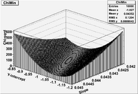
As shown above, I have plotted the value of [math]\chi^2[/math] as a function of the y-Intercept [math](a_1)[/math] and the slope [math](a_2)[/math]. The minimum in this hypersurface should coincide with the values of Y-intercept=[math]a_1=-1.01[/math] and Slope=[math]a_2=0.0431[/math] from the linear regression solution.

If we return to the beginning, the original problem is to use the max-likelihood principle on the probability function for finding the correct fit using the data.

[math]P(a_0,a_1, \cdots ,a_n) = \Pi_i P_i(a_0,a_1, \cdots ,a_n) =\Pi_i \frac{1}{\sigma_i \sqrt{2 \pi}} e^{- \frac{1}{2} \left ( \frac{y_i - y(x_i)}{\sigma_i}\right)^2} \propto e^{- \frac{1}{2}\left [ \sum_i^N \left ( \frac{y_i - y(x_i)}{\sigma_i}\right)^2 \right]}[/math]

Let

[math]\chi^2 = \sum_i^N \left ( \frac{y_i -y(x_i)}{\sigma_i}\right )^2[/math]

where [math]N[/math] = number of data points and [math]n[/math] = order of polynomial used to fit the data.

To maximize the probability of finding the best fit we need to find by minimum in [math]\chi^2[/math] by setting the partial derivate with respect to the fit parameters [math]\left (\frac{\partial \chi}{\partial a_k} \right)[/math] to zero

[math]\frac{\partial \chi^2}{\partial a_k} = \frac{\partial}{\partial a_k}\sum_i^N \frac{1}{\sigma_i^2} \left ( y_i - y(x_i)\right )^2[/math]

[math]= \sum_i^N 2 \frac{1}{\sigma_i^2} \left ( y_i - y(x_i)\right ) \frac{\partial \left( - y(x_i) \right)}{\partial a_k} = 0[/math]

Alternatively you could also express \chi^2 in terms of the probability distributions as

[math]P(a_0,a_1, \cdots ,a_n) \propto e^{- \frac{1}{2}\chi^2}[/math]

[math]\chi^2 = -2\ln\left [P(a_0,a_1, \cdots ,a_n) \right ] + 2\sum \ln(\sigma_i \sqrt{2 \pi})[/math]

Grid search method

The grid search method relies on the independence of the fit parameters [math]a_i[/math]. The search starts by selecting initial values for all parameters and then searching for a [math]\chi^2[/math] minimum for one of the fit parameters. You then set the parameter to the determined value and repeat the procedure on the next parameter. You keep repeating until a stable value of [math]\chi^2[/math] is found.

Obviously, this method strongly depends on the initial values selected for the parameters.

Parameter Errors

Returning back to the equation

[math]\chi^2 = -2\ln\left [P(a_0,a_1, \cdots ,a_n) \right ] + 2\sum \ln(\sigma_i \sqrt{2 \pi})[/math]

it may be observed that [math]\sigma_i[/math] represents the error in the parameter [math]a_i[/math] and that the error alters [math]\chi^2[/math].

Once a minimum is found, the parabolic nature of the [math]\chi^2[/math] dependence on a single parameter is such that an increase in 1 standard deviation in the parameter results in an increase in [math]\chi^2[/math] of 1.

We can turn this to determine the error in the fit parameter by determining how much the parameter must increase (or decrease) in order to increase [math]\chi^2[/math] by 1.

Gradient Search Method

The Gradient search method improves on the Grid search method by attempting to search in a direction towards the minima as determined by simultaneous changes in all parameters. The change in each parameter may differ in magnitude and is adjustable for each parameter.

Go Back Forest_Error_Analysis_for_the_Physical_Sciences#Statistical_inference