|
|
| Line 169: |
Line 169: |
| | | | |
| | :<math>\Rightarrow</math> | | :<math>\Rightarrow</math> |
| − | ::V_{out}^P = \frac{CR_{\parallel}}{RC}V_0 | + | ::<math>V_{out}^P = \frac{CR_{\parallel}}{CR_1}V_0</math> |
| | | | |
| | [[Forest_Electronic_Instrumentation_and_Measurement]] | | [[Forest_Electronic_Instrumentation_and_Measurement]] |
Revision as of 05:31, 9 February 2011
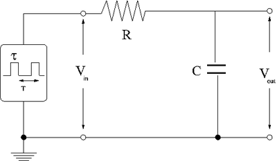
Differentiator circuit
Consider the effect of a low-pass filter on a rectangular shaped input pulse with a width [math]\tau[/math] and period [math]T[/math].
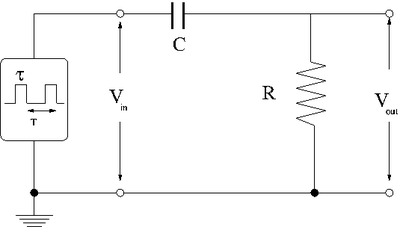
The first thing to consider is what happens to the different parts of the square pulse as it travels to the circuit.
You know that the circuit, as a high pass filter, will tend to attenuate low frequency (slow changing) voltages and not high frequency (quick changing) voltages.
This means no DC voltage values pass beyond the capacitor.
This means that points [math]a[/math] and [math]b[/math] in the pulse shown below should pass through the circuit.
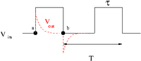
The voltage changes in between point [math]a[/math] and DC are passed according to what you select for the break frequency ([math]\omega_B = \frac{1}{RC}[/math])
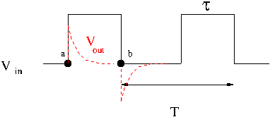
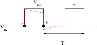
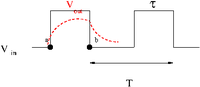
In the above pulse picture it was assumed that [math]\tau \gt \gt \frac{1}{\omega_B} = RC[/math] or in other words the RC network time constant is a lot smaller than the pulse width.
If the RC time constant is larger than the pulse width then you will see the voltage stay high. The rectangular pulse will be output as a square like pulse which is "sagging".
 |
|
| [math] RC \lt \lt \tau[/math] |
[math]RC \gt \gt \tau[/math]
|
Loop Theorem
- [math]V_{in} = V_C + V_R = I X_C + I R[/math]
- How does [math]V_C[/math] compare to [math]V_R[/math] ?
- [math]\left | \frac{V_R}{V_C} \right | = \frac{\left | IR \right |}{\left | I X_C\right |}= \frac{R}{\left | \frac{1}{i \omega C}\right |} = \omega RC[/math]
The maximum value of [math]\omega[/math] is determined by the pulse width [math] \tau[/math] while [math]T[/math] is the period that corresponds the lowest frequency (other than DC).
- [math]\left | \frac{V_R}{V_C} \right |_{MAX} = \frac{RC}{\tau}[/math]
[math]RC \lt \lt \tau[/math]
When [math]RC \lt \lt \tau[/math]
- [math]\left | \frac{V_R}{V_C} \right |_{MAX} = \frac{RC}{\tau} \lt \lt 1 \Rightarrow V_R [/math] may be ignored.
- [math]\Rightarrow V_{in} = V_C + V_R \approx V_C = \frac{Q}{C}[/math]
taking the derivative with respect to time yields
- [math]\frac{d V_{in}}{dt} = \frac{I}{C}[/math]
or
- [math]I = C \frac{d V_{in}}{dt}[/math]
The loop theorem for V_{out} :
- [math]V_{out} = IR = \left ( C \frac{d V_{in}}{dt} \right ) R = RC \frac{d V_{in}}{dt}[/math]
The output of the above circuit when [math]RC \lt \lt \tau[/math] will be proportional to the derivative of the input AC source with respect to time.
Integrator
The above circuit is a low pass filter. When a square pulse hits it all of the low frequency components will pass through and the high frequency components will be attenuated. This essentially makes the pulse smooth as shown below.
The above is referred to as an integration circuit.
Loop theorem
- [math]V_{in} = IR + \frac{Q}{C}[/math]
- [math]= R \frac{dQ}{dt} + \frac{Q}{C}[/math]
This differential equation may be written as
- [math]\frac{dQ}{dt} + \frac{Q}{RC} = \frac{V_{in}}{R}[/math]
- [math]\Rightarrow Q = CV_{in} \left (1 - e^{-t/RC} \right)[/math]
- [math]V_{out} = \frac{Q}{C} = V_{in}\left (1 - e^{-t/RC} \right)[/math]
[math]RC \gt \gt \tau[/math]
If [math]RC \gt \gt \tau[/math]
then
- [math]t/RC \lt \lt 1[/math]
- [math]e^{-t/RC} \approx 1- t/RC[/math]
- [math]\Rightarrow V_{out} = V_{in}\left (1 - e^{-t/RC} \right) = V_{in} \frac{t}{RC} = \frac{1}{RC} \int_0^t V_{in} dt[/math] The circuit appears to be integrating the input voltage.
If [math]RC \lt \lt \tau[/math] then very little integration is done because the pulse is change at a low frequency compared to the RC constant.
Pulse Sharpening
The circuit below is a way to decrease the rise time of an input pulse at the expense of attenuating the pulse. The output pulse is a "sharpened" version of the input pulse and attenuated.
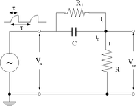
Junction Rule
If we apply the junction rule for the currents in the above circuit
Then
- [math]I_1 +I_2 = I[/math]
- [math]I_1 = \frac{V_{in}-V_{out}}{R_1}[/math]
- [math]I_2 = \frac{d}{dt} C\left( V_{in}-V_{out}\right) : Q =C \Delta V = C\left( V_{in}-V_{out}\right)[/math]
- [math]I = \frac{V_{out}}{R}[/math]
- [math]\Rightarrow[/math]
- [math]\frac{V_{in}-V_{out}}{R_1} + \frac{d}{dt} C\left( V_{in}-V_{out}\right) = \frac{V_{out}}{R}[/math]
Collecting terms
- [math]\frac{V_{in}}{R_1} + \frac{d}{dt} C\left( V_{in}\right) = \frac{d}{dt} C\left( V_{out}\right) + \frac{V_{out}}{R} + \frac{V_{out}}{R_1} [/math]
- [math]\frac{d V_{in} }{dt}+ \frac{V_{in}}{CR_1}= \frac{dV_{out}}{dt} + \frac{(R+R_1)}{CRR_1} V_{out} [/math]
assuming
- [math]V_{in} = V_0 \left ( 1-e^{-t/\tau_{in}}\right )[/math]
- [math]\Rightarrow[/math]
- [math]\frac{dV_{out}}{dt} + \frac{(R+R_1)}{CRR_1} V_{out} = V_0 \left ( \frac{1}{\tau_{in}} - \frac{1}{CR_1}\right )e^{-t/\tau_{in}} + \frac{V_0}{CR_1} [/math]
If [math]CR_1 = \tau_{in}[/math]
Then
- [math]\frac{dV_{out}}{dt} + \frac{(R+R_1)}{CRR_1} V_{out} = \frac{V_0}{CR_1} = Constant[/math]
The above is a first order non-homogeneous differential equation
To solve you first find a solution to the homogeneous equation ([math]V_{out}^H)[/math] and then form a particular solution [math](V_{out}^P)[/math] based on the homogeneous solution
Homogeneous Solution
- [math]\frac{dV_{out}^H}{dt} + \frac{(R+R_1)}{CRR_1} V_{out}^H = 0[/math]
- [math]\Rightarrow \frac{dV_{out}^H}{dt} = - \frac{(R+R_1)}{CRR_1} V_{out}^H \equiv \frac{1}{CR_{\parallel}} V_{out}^H[/math]
- [math] V_{out}^H = D e^{-t/CR_{\parallel}}[/math]
Particular Solution
- [math]\frac{dV_{out}}{dt} + \frac{(R+R_1)}{CRR_1} V_{out} = \frac{V_0}{CR_1} = Constant[/math]
- [math]V_{out} = V_{out}^P + V_{out}^H[/math]
- [math] V_{out}^H = D e^{-t/CR_{\parallel}}[/math]
- [math]\Rightarrow[/math]
- [math]V_{out}^P = \frac{CR_{\parallel}}{CR_1}V_0[/math]
Forest_Electronic_Instrumentation_and_Measurement


