TF EIM Chapt2

Alternating Current (AC)

Thus far we have discussed direct current circuits which were built from a battery (constant voltage supply).

Another type of circuit is one in which the current is driven in an alternating fashion. Typically the current is increased so some positive maximum value, then decreased until it passes through zero and reverses direction until it reaches another maximum value and then it is decreased again, passing though zero once more on its way to a positive maximum value.

Definitions

frequency ([math]f[/math], [math]\nu[/math] )

The frequency is number of complete cycles which occur in 1 sec (cycles/sec = Hz)

Angular frequency =[math] \omega = 2\pi f[/math] = radians/sec

Period

The period is the time to complete one cycle = 1/[math]f[/math]

Amplitude

The change in the current from zero to its most positive value

peak-to-peak

The amount the current changes from its largest positive value to its most negative.

phase

The time a current takes to reaches its maximum value compared to another alternating current

Note

The above definitions can be used for voltage as easily as current.

Mathematical description

Trigonometric

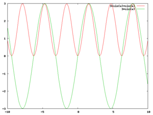
[math]I(t) = \sin(\omega t + \phi) = \cos(\omega t + \phi - \pi/2)[/math]

Note

A 180 degree ([math]\pi[/math] radian) phase shift will put the above cosine wave completely out of sync with the original one such that if we add the two signals together the net current would be zero.

I_{RMS}

With this functional form for the alternating current we can now calculate another property, the RMS or root mean square.

The RMS quantifies an average fluctuation of the alternating current such that

[math]I_{RMS} \equiv \sqrt{\frac{1}{T} \int_0^T I^2(t) dt} = \sqrt{\frac{1}{T} \int_0^T I_0^2 \sin^2(\omega t) dt}= \frac{I_0}{\sqrt{2}} [/math]

where T represent the time interval over which the average is calculated ([math]\infty[/math])

[math]\int_0^T \sin^2(x) dx = \int_0^T \frac{1}{2} \left (1 - \cos(2x) \right) dx = \frac{1}{2} + \frac{1}{T} \int_0^T \cos(t)dt = \frac{1}{2}[/math] if T is infinite or an integer number of cycles

Power

The instantaneous power dissipated in a resister by an alternating current is given as

[math]P_{inst}(t) =I^2(t) R = R\sin^2(\omega t)[/math]

Average power

[math]P_{ave} = \frac{1}{T} \int_0^T P(t) dt = \frac{1}{T} \int_0^T RI^2(t) dt = \frac{R}{T} \int_0^T \sin^2(\omega t) dt = \frac{I_0^2R}{\sqrt{2}} = I_{RMS}^2 R[/math]

Plane waves

Another mathematical expression for an alternating current uses complex variables

[math]I\left ( \omega t \right )=I_0 \exp^{i \left ( \omega t \right )} = I_0 \left ( \cos \left ( \omega t \right) + i \sin \left ( \omega t \right) \right )[/math]

Expressing the current in this form will be useful later

Voltage sources of AC current

The circuit symbol for an emf used to drive alternating currents is given below

A mathematical form is for an AC voltage source is:

[math]V = V_0 \sin(\omega t)[/math]

Capacitors

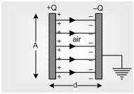
A capacitor is a device used to store charge in a circuit. The simplest capacitor is built from two conducting plates placed close to each other.

Notice

The potential is constant over the face of the capacitor

[math]V_{AB} = - \int_A^B \vec{E} \cdot d \vec{l}[/math]

The symbol for a capacitor in a circuit is usually.

or

electrolytic symbol

The electrolytic capacitor

Electrolytic capacitors can be shorted out. Put the positive probe from the voltmeter on the positive side of the electrolytic capacitor, the capacitor should be good if you measure a large resistance [math](k \Omega)[/math] otherwise a shorted electrolytic capacitor (small resistance) is a bad one.

Capacitor Properties

1. [math]C\gt 0[/math] Measures ability to store charge
2. [math]V=Q/V[/math] : Double Q Doubles V
3. SI units = Farrads = Coul/Volt
4. Magnitude depends on the elements geometry (conductor area, separation of conductors, ...)

Capacitors in Parallel and Series

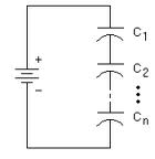
Series

Capacitors in Series add like resistors in Parallel.(Capacitance decreases when hooked up in series)

Note

The same amount of charge is pushed onto each capacitor

For capacitors in series you can apply the loop theorem for the above case and the one where all the capacitors are replaced by a single capacitor.

[math]V_{tot} = V_1+V_2+ ...[/math]

[math]Q/C_{tot} = Q/C_1+Q/C_2+ ...[/math]

[math]1/C_{tot} = 1/C_1+1/C_2+ ...[/math]

Parallel

Capacitors in parallel add like resistors in Series (Capacitance increases when hooked up in parallel)

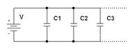
If you were to replace all capacitors with an equivalent capacitance (C_{eq}) then the charge driven onto the equivalent capacitance would be equal to the sum of the charge driven onto each capacitor.

[math]Q_{tot} = Q_{eq} = Q_1 + Q_2 +[/math] ...

[math]VC_{tot} = VQ_{eq} = VQ_1 + VQ_2 +[/math] ...

[math]C_{tot} = Q_{eq} = Q_1 + Q_2 +[/math] ...

Charging/Discharging Capacitor circuit

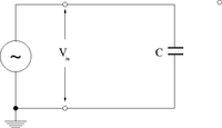
If

[math]V=V_0 cos(\omega t)[/math]

then applying loop theorem lead to

[math]V-\frac{Q}{C} = 0[/math]

[math]Q = VC= V_0 C \cos{\omega t)}[/math]

[math]I = \frac{dQ}{dt} = -V_0C \omega \sin(\omega t)= V_0 C \omega \cos(\omega t + \pi/2)[/math]

Notice that the current is 90 degrees out of phase with the driving voltage.

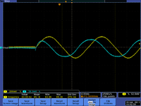
Phase shift using 562nF capacitor and a 200 mV sine wave voltage source at 65 Hz

Note

The current increases faster than the voltage. Below are a few scope pictures measuring the voltage coming out of the voltage source [math](V_{in})[/math] and the voltage on the ground side of the capacitor [math](V_{out})[/math] (the capacitor is grounded through the scope). This is actually a high pass filter because of the internal resistance of the scope used to measure [math]V_{out}[/math].

1 Hz	16Hz	kHz
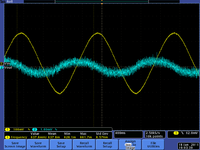Capacitor response at low frequency	16Hz frequency	kHz frequency

Reactance: Resistive nature of capacitance

To illustrate the resistive nature of capacitors, let's write the driving voltage in using complex notation

[math]V=V_0 \cos(\omega t) = V_0 Re \left [ e^{i\omega t} \right ][/math]

The notation

[math] e^{\omega t} = \cos(\omega t) + i \sin(\omega t)[/math]: Euler's equation

[math] Re \left [ e^{i\omega t} \right ]=Re \left [ \cos(\omega t) + i \sin(\omega t) \right ]= \cos(\omega t) [/math] The real part of a complex variable.

The current is written as

[math]I=\omega CV_0 Re \left [ e^{i \left (\omega t + \pi/2 \right ) } \right ][/math]

[math] =\omega C V_0 Re \left [ e^{i \left ( \omega t \right )} e^{i \left ( \pi/2 \right )} \right ][/math]

[math] =\omega C V_0 Re \left [ e^{i \left ( \omega t \right )} \left ( \cos(\pi/2) + i sin(\pi/2) \right ) \right ][/math]

[math] =\omega C V_0 Re \left [ e^{i \left ( \omega t \right )} \left ( 0 + i \right )\right ][/math]

[math] =\omega C V_0 Re \left [ i e^{i \left ( \omega t \right )} \right ][/math]

[math] =Re \left [ V_0 \frac{e^{i \left ( \omega t \right )}}{\frac{1}{i\omega C}} \right ]=Re \left [ V_0 \frac{e^{i \left ( \omega t \right )}}{X_C} \right ][/math]

where

[math]X_C = \frac{1}{i \omega C}[/math] Effective impedance of a Capacitor

Observe

At high frequencies [math](\omega)[/math] the effective impedance (X_C) is small so the driving voltage should pass right through.

At low frequencies [math](\omega)[/math] the effective impedance (X_C) is large so the driving voltage will be severely attenuated.

Capacitors block Alternating Currents so you can reduce ripples on DC voltages.

You could measure the capacitance by measuring [math](I/V)^2[/math] for several frequencies

RC circuit

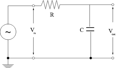
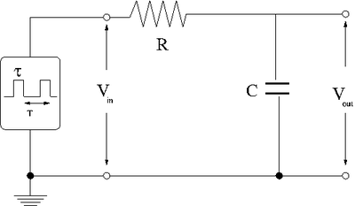
The Low pass Fiter

Now add a resistor in series with the capacitor in the above capacitor charging circuit so it resembles the circuit below

Quick Solution

Applying the loop theorem using the reactance[math] X_C[/math] of the capacitor instead of Q/C

[math]V - IR -X_CI = =V -(X_R +X_C) I = 0[/math]

[math]\Rightarrow[/math] the capacitor can be added in series with the other resistor

[math]X_{tot} = X_R + X_C[/math]

It looks like the voltage divider from the resistance section

[math]V_{out}= Re\left [\frac{X_C}{R+X_C} V_{in} \right ]= Re \left [\frac{X_C}{X_R+X_C} V_{in} \right ][/math]

To evaluate [math]Re[Z] = \sqrt{Z Z^*}[/math] where[math] Z = x+iy[/math] and [math]Z^* = x-iy[/math]

[math]\frac{V_{out}}{V_{in}} = Re \left [ \frac{\frac{1}{i \omega C}}{R+\frac{1}{i \omega C}} \right ] = \sqrt{\frac{\frac{1}{i \omega C}}{R+\frac{1}{i \omega C}} \frac{\frac{1}{-i \omega C}}{R+\frac{1}{-i \omega C}} } = \frac{1}{\sqrt{1 + \omega^2 R^2 C^2}}[/math]

Let

[math]\omega_b = \frac{1}{RC} =[/math] break point (cut off ) frequency

then

[math]\frac{V_{out}}{V_{in}} = \frac{1}{\sqrt{1 + \left ( \frac{\omega}{\omega_b}\right )^2}}[/math]

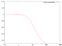
Note

The RC circuit is another way to measure the capacitance by measureing [math]V_{out}/V_{in}[/math] -vs- [math]\omega[/math] and do a linear extrapolation to determine the break point frequency.

Phasor Diagram

Phasor diagrams are a technique used to illustrate the phase difference between the input and output alternating voltages/currents.

Returning to the loop theorem for the low pass RC filter

[math]V_{in} = V_R + V_{out}[/math]

[math]V_{in} = IX_R + IX_C[/math]

[math]V_{in} = IR + I\frac{-i}{\omega C}[/math]

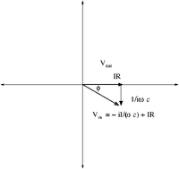
We can write the voltage as a complex variable using a coordinate system in which the "x-axis" represents real numbers and the "y-axis" represents the complex components. This is analogous to expressing 2-D vectors.

Below is a figure representing the complex plane.

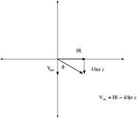
The angle [math]\phi[/math] is the angle between[math] V_{out} = \frac{-i}{\omega C}[/math] and [math]V_{in} = IR + I\frac{-i}{\omega C}[/math] Based on the above Phasor diagram

[math]\tan(\phi) = \left (\frac{R}{\frac{-1}{\omega C}} \right )= \left(\omega RC \right )[/math]

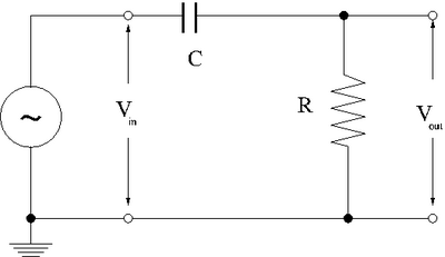
High Pass Filter

A high pass filter switches the order of the resistor and the capacitor.

Using the same reactance based analysis as above

[math]V_{in} - IX_C - IR = 0[/math]

[math]V_{out} = IR[/math]

[math]\frac{V_{out}}{V_{in}} = \frac{IR}{I \left ( X_C + R \right ) }= \frac{R}{\frac{1}{i \omega C} + R} = \frac{ i \omega RC}{1 + i \omega RC}[/math]

[math]\left |\frac{V_{out}}{V_{in}} \right | = \sqrt{\left ( \frac{ i \omega RC}{1 + i \omega RC}\right ) \left ( \frac{- i \omega RC}{1 - i \omega RC}\right )} = \frac{\omega RC}{\sqrt{(1 + \omega^2 R^2C^2}}[/math]

Phasor diagram

The phasor diagram is very similar except this time V_{out} is along the x-axis

Returning to the loop theorem for the low pass RC filter

[math]V_{in} = V_R + V_{out}[/math]

[math]V_{in} = IX_C + IX_R [/math]

[math]V_{in} = I\frac{-i}{\omega C}+IR[/math]

We can write the voltage as a complex variable using a coordinate system in which the "x-axis" represents real numbers and the "y-axis" represents the complex components. This is analogous to expressing 2-D vectors.

Below is a figure representing the complex plane.

The angle [math]\phi[/math] is the angle between [math]V_{out} =IR[/math] and [math]V_{in} = I\frac{-i}{\omega C} + IR [/math] Based on the above Phasor diagram

[math]\tan(\phi) = \left (\frac{\frac{-1}{\omega C}}{R} \right ) = (\frac{-1}{\omega RC})[/math]

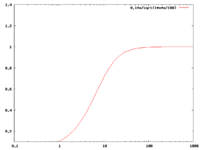
High Pass -vs- Low Pass graphs

if

[math]\omega_B=\frac{1}{RC}=10[/math]

Low pass	High Pass
Gain -vs- [math]\omega[/math]	Gain -vs- [math]\omega[/math]
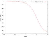Phase Shift -vs- [math]\omega[/math]	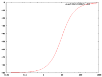Phase Shift -vs- [math]\omega[/math]

exact solution

Again apply the loop theorem

[math]V -IR -\frac{Q}{C} =0[/math]

or

[math]R \frac{dQ}{dt} + \frac{1}{C} Q =V(t)[/math] First order non-homogeneous linear differential equation

First solve homogeneous part

[math]R \frac{dQ}{dt} + \frac{1}{C} Q =0[/math] First order homogeneous linear differential equation

The above is integratable

[math] \frac{dQ}{dt} = -\frac{1}{RC} Q [/math]

[math]\int \frac{dQ}{Q} = -\int \frac{1}{RC} dt [/math]

[math]\ln Q = -\frac{t}{RC} -Constant[/math]

[math] Q(t) = e^{-\frac{t}{RC}} e^{Constant} = Q_0e^{-\frac{t}{RC}}[/math]

[math] I(t)= \frac{d Q}{d t} = \frac{d}{dt} Q_0 e^{-\frac{t}{RC}} = \frac{-Q_0}{RC}e^{-\frac{t}{RC}}[/math]

This gives you the general solution for the homogeneous problem

In this case it represents the solution for a discharging capacitor.

Trial solution method for Non-Homogeneous Solution

A common and more general technique to solving such a differential equation is to use the solution from the discharging equation (the homogeneous diff. eq.) as a trial solution by inserting constants.

[math]Q_{trial} = A + Be^{-t/RC}[/math]

You then substitute this trial solution into the differential equation and apply boundary conditions to determine the coefficients.

[math]\frac{d}{dt} \left ( A + Be^{-t/RC} \right ) + \frac{1}{RC} \left ( A + Be^{-t/RC} \right ) = \frac{dV}{Rdt}[/math]

[math] \left ( B \frac{-1}{RC}e^{-t/RC} \right ) + \frac{1}{RC} \left ( A + Be^{-t/RC} \right ) = \frac{dV}{Rdt}[/math]

[math]\Rightarrow \frac{1}{RC} \left ( A \right ) = \frac{dV}{Rdt}[/math]

[math]A = C \frac{dV}{dt} = C \frac{d V_0 e^{i \omega t}}{dt}[/math]

To determine the other coefficient you apply the boundary condition that q = 0 when t=0

[math]0= A + Be^{-0/RC} = A+B[/math]

[math]A=-B[/math]

[math]Q=CV (1 - e^{-t/RC}) =Q_0 (1 - e^{-t/RC})[/math]

Inductance

Inductor/Choke

An inductor is basically a loop of wire wrapped around a core (or air) to form a coil.

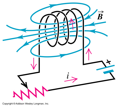
Consider what happens in the above circuit when you first connect a voltage source (or close the switch).

1.) A current starts to flow through the wire such that I=V/R (R can be the internal resistance of the battery which changes with time).

2.) A current produces a magnetic field

Ampere's Law

[math]\oint \vec{B} \cdot d \vec{l} = \mu_0 I[/math]

If the current distribution isn't symmetric enough to make the line integral easy

then you may need to use

Biot-Savart Law

[math]d\vec{B} = \frac{\mu_0 I}{4 \pi} \frac{\vec{l} \times \vec{r}}{r^2}[/math]

Most inductors take the geometrical form of a solenoid.

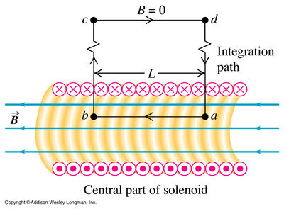
[math]\oint \vec{B} \cdot \vec{l} = \int_a^b \vec{B} \cdot d\vec{l} + \int_b^c \vec{B} \cdot d\vec{l} + \int_c^d \vec{B} \cdot d\vec{l} + \int_d^a \vec{B} \cdot d\vec{l} = \mu_0 I_{tot}[/math]

[math]\int_a^b \vec{B} \cdot d\vec{l} = B\ell[/math]

[math]\int_b^c \vec{B} \cdot d\vec{l} = \int_d^a \vec{B} \cdot d\vec{l} =0 : \vec{B} \perp d\vec{l}[/math]

[math]\int_c^d \vec{B} \cdot d\vec{l} =0 : B \approx 0[/math]

[math] I_{tot} = NI[/math] = total current enclosed by the loop is I times the number of loops N

[math]B = \mu_0 \frac{NI}{\ell} = \mu_0 nI[/math]

where

[math]n \equiv \frac{N}{\ell} =[/math] number of turns per unit length

3.) When using an AC source the current is changing with time and as a result the B-field is also changing in time

4.) The changing current induces and emf ([math]\mathcal{E}[/math])

Faraday's law of induction says

[math]\mathcal{E} = - \frac{d \Phi_B}{dt}[/math] = self induced emf

where

[math]\Phi_B = \int \vec{B} \cdot d \vec{A}[/math]

[math]\mathcal{E} = - \frac{d }{dt} \int \vec{B} \cdot d \vec{A}[/math]: There are 3 ways to induce an emf (B and A change with time or the angle between them)

The B-field is usually perpendicular to the area of the induction and mostly uniform.

[math]\mathcal{E} = - \frac{d }{dt} BA = - \frac{d }{dt} \mu_o nIA = - \mu_0nA \frac{dI}{dt} [/math]

The above is the emf induced in a single loop

If you assume there are N loop in the inductor

Then

[math]\mathcal{E} = - N\frac{d }{dt} \mu_o nIA = - N\mu_0nA \frac{dI}{dt} \equiv -L \frac{dI}{dt}[/math]

[math]L = N\mu_0 n A = \mu_0 \frac{N^2}{\ell} \pi R^2[/math] = Inductance

where

[math]\ell=[/math] length of loop

[math]R =[/math] radius of coil

Lenz's law says that the induced current will appear in a direction that opposes the change producing it.

So in essence the inductor acts "like" a resistor which resists the current flow according to the amount of current is changing.

There is an effective impedance [math]Z_{L}[/math] for inductors as there was one for capacitors

Inductor Reactance

Consider an AC voltage source with an inductor attached.

Loop theorem

[math]\Rightarrow V - L \frac{dI}{dt} = 0[/math]

[math]V_0 cos(\omega t) dt = L dI[/math]

[math]\int_0^t V_0 cos(\omega t) dt =\int_0^t L dI[/math]

[math]\left . V_0 \frac{sin(\omega t)}{\omega} \right |_o^t = L \left . I(t)\right |_0^t[/math]

[math]V_0 \frac{sin(\omega t)}{\omega} -0 = L \left ( I(t) - I(0)\right )[/math]

[math]\Rightarrow I(t) = V_0 \frac{sin(\omega t)}{\omega L} + I(0)[/math]

Assum I(0) =0 and rewrite [math]\sin[/math] in terms of a phase shifted [math]\cos[/math]

[math]\Rightarrow I(t) = \frac{V_0}{\omega L} cos(\omega t - \pi/2) [/math] : V and I are 90 degrees out of phase

[math]= Re \left ( \frac{V_0}{\omega L} e^{i(\omega t - \pi/2)}\right )[/math]

[math]= Re \left ( \frac{V_0}{\omega L} e^{i(\omega t)} (-i)\right )[/math]

[math]= Re \left ( \frac{V_0}{i\omega L} e^{i(\omega t)}\right )[/math]

[math]X_L \equiv i\omega L[/math]

Note

Large L makes it hard to change current

Small L makes it easy to change current

parallel LC circuit (Band Stop/Notch Filter/ tank circuit)

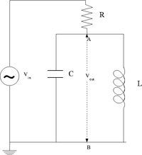
The above circuit has a resistor in series with an inductor and capacitor in parallel.

Using the complex analysis techniques for AC circuits you can consider the Inductor and Capacitor as impedances in parallel.

so

[math]\frac{1}{X_{tot}} = \frac{1}{X_C} + \frac{1}{X_L} = \frac{i \omega C}{1} + \frac{1}{i \omega L} = \frac{1- \omega^2 LC}{i \omega L}[/math]

[math] X_{tot} = \frac{i \omega L}{1- \omega^2 LC} = \frac{i \omega L}{1- \frac{\omega^2}{\omega_{LC}^2}}[/math]

[math]\omega_{LC} \equiv \frac{1}{\sqrt{LC}}[/math]

or

[math]\nu_{LC} = \frac{\omega_{LC}}{2\pi}\frac{1}{2 \pi \sqrt{LC}}[/math]

[math]L = 33 \mu H[/math] and [math]C = 1 \mu F [/math]

[math]\Rightarrow \omega = 174077.66[/math] rad/s

Phase differences

Notice

[math]X_C = \frac{1}{i \omega C}[/math] & [math]X_L = i \omega L[/math]

[math]I = \frac{V}{X}[/math]

[math]I_C = \frac{V}{\frac{1}{i \omega C}} = i \omega CV[/math]

[math]I_L = \frac{V}{i \omega L} = \frac{-iV}{\omega L }[/math]

The current through the inductor side of the circuit is 180 degrees out of phase with the capacitor side.

gain

Loop Theorem

[math]\Rightarrow V= I(R+X_{tot}) = I \left (R+ \frac{i \omega L}{1- \frac{\omega^2}{\omega_{LC}^2}} \right )[/math]

or

[math] I= \frac{V_0 e^{i \omega t}}{\left (R+ \frac{i \omega L}{1- \frac{\omega^2}{\omega_{LC}^2}} \right )}[/math]

Notice

When [math]\omega \approx \omega_{LC} = \sqrt{\frac{1}{LC}}[/math] then the AC signal is attenuated.

Looking at the Voltage divider aspect of the circuit

[math]V_{AB}=V_{out} = \frac{X_{tot} }{R + X_{tot}}V_{in}[/math]

[math]\left |\frac{ V_{out}} {V_{in}}\right | = \sqrt{ \left [ \frac{X_{tot} }{R + X_{tot}} \right ] \left [ \frac{X_{tot} }{R + X_{tot}} \right ]^*}[/math]

[math] = \sqrt{ \left [ \frac{\frac{i \omega L}{1- \frac{\omega^2}{\omega_{LC}^2}} }{\left (R+ \frac{i \omega L}{1- \frac{\omega^2}{\omega_{LC}^2}} \right )} \right ] \left [ \frac{\frac{i \omega L}{1- \frac{\omega^2}{\omega_{LC}^2}} }{\left (R+ \frac{i \omega L}{1- \frac{\omega^2}{\omega_{LC}^2}} \right )} \right ]^*}[/math]

[math] = \sqrt{ \frac{ \omega^2 L^2 \omega_{LC}^4}{R^2(\omega_{LC}^2 - \omega^2)^2 - \omega^2L^2 \omega_{LC}^4}}[/math]

[math] = \sqrt{ \frac{ \omega^2 }{C^2R^2(\omega_{LC}^2 - \omega^2)^2 - \omega^2}}[/math]

[math] = \sqrt{ \frac{ \omega^2 }{\frac{1}{\omega_{RC}^2}(\omega_{LC}^2 - \omega^2)^2 - \omega^2}}[/math]

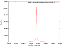
[math]L = 33 \mu H[/math] and [math]C = 1 \mu F [/math] and R=200 [math]\Omega[/math]

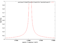
[math]\Rightarrow \omega = 174077.66[/math] rad/s or [math]\nu = \frac{\omega}{2 \pi} = 27705[/math] Hz

Q and Bandwidth

In the above circuit

[math]\nu = \omega/2 \pi = \frac{1}{2 \pi \sqrt{LC}}= 27705 Hz[/math]

The inductors reactance at this resonance frequency is

[math]X_{L} = \omega L = 2 \pi \nu L = \frac{L}{\sqrt{LC}} = \sqrt{\frac{L}{C}} = \sqrt{\frac{33 \times 10^{-6} H}{1 \times 10^{-6}F}} = 5.7 \Omega[/math]

Bandwith

The most common definition for the Bandwidth of this circuit is the frequency range over which the output decreases by 3 dB. This correspond to the frequency at which the circuits power is cut in half from the resonance frequency.

[math]P = I^2 R[/math]

[math]P_{1/2} = (\frac{1}{\sqrt{2}}I)^2 R= \frac{(\frac{1}{\sqrt{2}} V)^2}{R}[/math]

[math]\Rightarrow V = \frac{1}{\sqrt{2}} V = 0.71 V[/math]

The Band Width is a measurement of the two frequencies which will decrease the resonance voltage by 30 %.

Quality Factor

The Quality factor for this circuit may be expressed in term of the bandwidth such that

[math]Q=\frac{\omega_0}{BW}=\frac{\omega_0}{\Delta \omega}[/math]

Notice

The Bandwidth can be changed in the above circuit by changing the step down resistor (R) without changing the resonance frequency.

Quality Factor (Q)

The Quality factor of a circuit is defined in terms of a ratio between the energy stored to the energy lost.

[math]Q \equiv 2 \pi \frac{\mbox{Energy Stored per cycle}}{\mbox{Energy lost per cycle}} = 2 \pi \frac{W_S}{W_L}[/math]

How much energy does an inductor store?

[math]W = \mbox{Work} = \int \vec{F} \cdot d\vec{r} = \Delta U = \int V dQ = \int L \frac{d I}{dt} (I dt) = L \int_0^I I dI = \frac{1}{2} LI^2[/math]

[math]W_S = \frac{1}{2} LI^2[/math]

How much energy does an inductor lose?

The system loses energy through heat via power dissipation so in general

[math]W_L = \int p(t) dt = \int_0^T I^2(t) R dt [/math] where R is the effective resistance of the circuit

Note

A circuit with high Q will have amplitude (or blocking) at the desired resonance frequency and the least amplitude (or blocking) at non-resonant frequencies.

An Inductor in series with a capacitor is known as a Band Pass filter. Since wires are used to hook everything up and real capacitors have leakage resistance so an RLC circuit is a realistic version of the series LC circuit.

RLC circuit

An RLC circuit is a Resistor, an Inductors, and a Capacitor in series with an electromotive force.

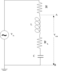
Effective impedance

[math]X_{out} = R_L + X_C + X_L = R_L + \frac{1}{i \omega C} + i \omega L[/math]

[math]\left | X_{out} \right | = \sqrt{\left [ R_L + i \left (\frac{-1}{\omega C} + \omega L\right ) \right ]\left [ R - i \left (\frac{-1}{\omega C} + \omega L\right ) \right ]^*}[/math]

[math]= \sqrt{ R_L^2 + \left ( \omega L - \frac{1}{\omega C} \right )^2}[/math]

Gain

Loop Theorem

[math]V_{in} = I (R+ X_{out})[/math]

Voltage Divider

[math]V_{AB}=V_{out} = \frac{X_{out}}{R + X_{out}}V_{in}[/math]

[math]\left | \frac{V_{out}}{V_{in}}\right | = \sqrt{\left [ \frac{X_{out}}{R + X_{out}}\right ]\left [ \frac{X_{out}}{R + X_{out}}\right ]^*}[/math]

[math]R_L + i \left ( \omega L - \frac{1}{\omega C}\right)[/math]

[math]\left | \frac{V_{out}}{V_{in}}\right | = \sqrt{\left [ \frac{R_L + i \left ( \omega L - \frac{1}{\omega C}\right)}{R + R_L + i \left ( \omega L - \frac{1}{\omega C}\right)}\right ]\left [ \frac{R_L + i \left ( \omega L - \frac{1}{\omega C}\right)}{R + R_L + i \left ( \omega L - \frac{1}{\omega C}\right)}\right ]^*}[/math]

[math] = \sqrt{\frac{R_L^2 + \left ( \omega L - \frac{1}{\omega C}\right)^2}{(R + R_L)^2 + \left ( \omega L - \frac{1}{\omega C}\right)^2}}[/math]

[math] = \sqrt{\frac{R_L^2 + \left ( \frac{\omega^2 LC - 1}{\omega C}\right)^2}{(R + R_L)^2 + \left ( \frac{\omega^2 LC - 1}{\omega C}\right)^2}}[/math]

Let

[math]\omega_0 = \sqrt{\frac{1}{LC}}[/math]

Then

[math]\left | \frac{V_{out}}{V_{in}}\right | = \sqrt{\frac{R_L^2 + \left ( \frac{\omega^2 - \omega_0^2}{\omega_0^2 \omega C}\right)^2}{(R + R_L)^2 + \left ( \frac{\omega^2- \omega_0^2}{\omega_o^2 \omega C}\right)^2}}[/math]

When[math] \omega = \sqrt{\frac{1}{LC}} = \omega_0[/math]

Then

[math]\left | \frac{V_{out}}{V_{in}}\right | =\frac{R}{R+R_L}[/math]

Phase shift

[math]X_C = \frac{-i}{\omega C} \Rightarrow[/math] Voltage lags current for a capacitor

[math]X_L = i \omega L \Rightarrow[/math] Voltage leads current for Inductor

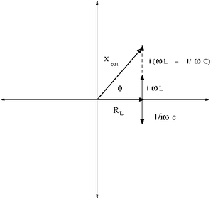
[math]\tan(\phi) = \frac{X_{out}}{R_L} = \frac{\omega L - \frac{1}{\omega C}}{R}= \frac{\omega^2 - \omega_o^2}{\omega_0^2R}[/math]

If [math]\omega \lt \omega_0[/math] then the phase shift is negative

If [math]\omega \gt \omega_0[/math] then the phase shift is positive

Differentiator circuit

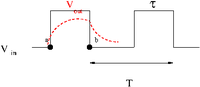
Consider the effect of a low-pass filter on a rectangular shaped input pulse with a width [math]\tau[/math] and period [math]T[/math].

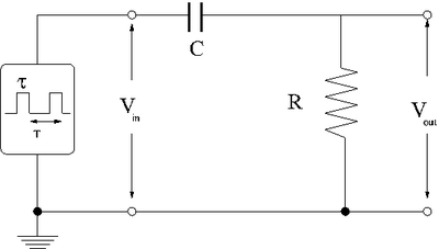
The first thing to consider is what happens to the different parts of the square pulse as it travels to the circuit.

You know that the circuit, as a high pass filter, will tend to attenuate low frequency (slow changing) voltages and not high frequency (quick changing) voltages.

This means no DC voltage values pass beyond the capacitor.

This means that points [math]a[/math] and [math]b[/math] in the pulse shown below should pass through the circuit.

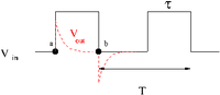
The voltage changes in between point [math]a[/math] and DC are passed according to what you select for the break frequency ([math]\omega_B = \frac{1}{RC}[/math])

In the above pulse picture it was assumed that [math]\tau \gt \gt \frac{1}{\omega_B} = RC[/math] or in other words the RC network time constant is a lot smaller than the pulse width.

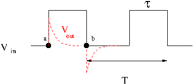
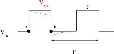
If the RC time constant is larger than the pulse width then you will see the voltage stay high. The rectangular pulse will be output as a square like pulse which is "sagging".

[math] RC \lt \lt \tau[/math]	[math]RC \gt \gt \tau[/math]

Loop Theorem

[math]V_{in} = V_C + V_R = I X_C + I R[/math]

How does [math]V_C[/math] compare to [math]V_R[/math] ?

[math]\left | \frac{V_R}{V_C} \right | = \frac{\left | IR \right |}{\left | I X_C\right |}= \frac{R}{\left | \frac{1}{i \omega C}\right |} = \omega RC[/math]

The maximum value of [math]\omega[/math] is determined by the pulse width [math] \tau[/math] while [math]T[/math] is the period that corresponds the lowest frequency (other than DC).

[math]\left | \frac{V_R}{V_C} \right |_{MAX} = \frac{RC}{\tau}[/math]

[math]RC \lt \lt \tau[/math]

When [math]RC \lt \lt \tau[/math]

[math]\left | \frac{V_R}{V_C} \right |_{MAX} = \frac{RC}{\tau} \lt \lt 1 \Rightarrow V_R [/math] may be ignored.

[math]\Rightarrow V_{in} = V_C + V_R \approx V_C = \frac{Q}{C}[/math]

taking the derivative with respect to time yields

[math]\frac{d V_{in}}{dt} = \frac{I}{C}[/math]

or

[math]I = C \frac{d V_{in}}{dt}[/math]

The loop theorem for V_{out} :

[math]V_{out} = IR = \left ( C \frac{d V_{in}}{dt} \right ) R = RC \frac{d V_{in}}{dt}[/math]

The output of the above circuit when [math]RC \lt \lt \tau[/math] will be proportional to the derivative of the input AC source with respect to time.

Integrator

The above circuit is a low pass filter. When a square pulse hits it all of the low frequency components will pass through and the high frequency components will be attenuated. This essentially makes the pulse smooth as shown below.

The above is referred to as an integration circuit.

Loop theorem

[math]V_{in} = IR + \frac{Q}{C}[/math]

[math]= R \frac{dQ}{dt} + \frac{Q}{C}[/math]

This differential equation may be written as

[math]\frac{dQ}{dt} + \frac{Q}{RC} = \frac{V_{in}}{R}[/math]

[math]\Rightarrow Q = CV_{in} \left (1 - e^{-t/RC} \right)[/math]

[math]V_{out} = \frac{Q}{C} = V_{in}\left (1 - e^{-t/RC} \right)[/math]

[math]RC \gt \gt \tau[/math]

If [math]RC \gt \gt \tau[/math]

then

[math]t/RC \lt \lt 1[/math]

[math]e^{-t/RC} \approx 1- t/RC[/math]

[math]\Rightarrow V_{out} = V_{in}\left (1 - e^{-t/RC} \right) = V_{in} \frac{t}{RC} = \frac{1}{RC} \int_0^t V_{in} dt[/math] The circuit appears to be integrating the input voltage.

If [math]RC \lt \lt \tau[/math] then very little integration is done because the pulse is change at a low frequency compared to the RC constant.

Pulse Sharpening

The circuit below is a way to decrease the rise time of an input pulse at the expense of attenuating the pulse. The output pulse is a "sharpened" version of the input pulse and attenuated.

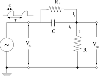
Junction Rule

If we apply the junction rule for the currents in the above circuit

Then

[math]I_1 +I_2 = I[/math]

[math]I_1 = \frac{V_{in}-V_{out}}{R_1}[/math]

[math]I_2 = \frac{d}{dt} C\left( V_{in}-V_{out}\right) : Q =C \Delta V = C\left( V_{in}-V_{out}\right)[/math]

[math]I = \frac{V_{out}}{R}[/math]

[math]\Rightarrow[/math]

[math]\frac{V_{in}-V_{out}}{R_1} + \frac{d}{dt} C\left( V_{in}-V_{out}\right) = \frac{V_{out}}{R}[/math]

Collecting terms

[math]\frac{V_{in}}{R_1} + \frac{d}{dt} C\left( V_{in}\right) = \frac{d}{dt} C\left( V_{out}\right) + \frac{V_{out}}{R} + \frac{V_{out}}{R_1} [/math]

[math]\frac{d V_{in} }{dt}+ \frac{V_{in}}{CR_1}= \frac{dV_{out}}{dt} + \frac{(R+R_1)}{CRR_1} V_{out} [/math]

assuming

[math]V_{in} = V_0 \left ( 1-e^{-t/\tau_{in}}\right )[/math]

[math]\Rightarrow[/math]

[math]\frac{dV_{out}}{dt} + \frac{(R+R_1)}{CRR_1} V_{out} = V_0 \left ( \frac{1}{\tau_{in}} - \frac{1}{CR_1}\right )e^{-t/\tau_{in}} + \frac{V_0}{CR_1} [/math]

If [math]CR_1 = \tau_{in}[/math]

Then

[math]\frac{dV_{out}}{dt} + \frac{(R+R_1)}{CRR_1} V_{out} = \frac{V_0}{CR_1} = Constant[/math]

The above is a first order non-homogeneous differential equation

To solve you first find a solution to the homogeneous equation ([math]V_{out}^H)[/math] and then form a particular solution [math](V_{out}^P)[/math] based on the homogeneous solution

Homogeneous Solution

[math]\frac{dV_{out}^H}{dt} + \frac{(R+R_1)}{CRR_1} V_{out}^H = 0[/math]

[math]\Rightarrow \frac{dV_{out}^H}{dt} = - \frac{(R+R_1)}{CRR_1} V_{out}^H \equiv \frac{1}{CR_{\parallel}} V_{out}^H[/math]

[math] V_{out}^H = D e^{-t/CR_{\parallel}}[/math]

Particular Solution

[math]\frac{dV_{out}}{dt} + \frac{(R+R_1)}{CRR_1} V_{out} = \frac{V_0}{CR_1} = Constant[/math]

[math]V_{out} = V_{out}^P + V_{out}^H[/math]

[math] V_{out}^H = D e^{-t/CR_{\parallel}}[/math]

[math]\Rightarrow[/math]

[math]V_{out}^P = \frac{CR_{\parallel}}{CR_1}V_0[/math]

Apply Boundary Conditions

[math]V_{out} =\frac{R_{\parallel}}{R_1}V_0 + D e^{-t/CR_{\parallel}}[/math]

[math]V_{out}(t=0) = 0 \Rightarrow D = - \frac{R_{\parallel}}{R_1}V_0[/math]

[math]V_{out} =\frac{R_{\parallel}}{R_1}V_0 (1- e^{-t/CR_{\parallel}})[/math]

[math]= \frac{R}{R+R_1}V_0 (1- e^{-t/\tau_{out}})[/math]

where

[math]\tau_{out} \equiv CR_{\parallel} = C \frac{RR_1}{R+R_1} =\frac{R}{R+R_1} \tau_{in} \lt \tau_{in} [/math]

Note

[math]\tau_{out}[/math] is always less than [math]\tau_{in}[/math]

or in other words the rise time of the output pulse is short than the rise time of the input pulse

or in other words the output pulse is sharper (rising faster) than the input pulse

[math]\frac{\tau_{out}}{\tau_{in}} = \frac{R}{R+R_1}[/math]

So the output pulse is faster by a factor of [math]\frac{R}{R+R_1}[/math] and attenuated by the same factor!

Forest_Electronic_Instrumentation_and_Measurement