Simulations of Particle Interactions with Matter
Class Admin
Forest_SimPart_Syllabus
The ability to simulate nature using a computer has become a useful skill for physicists who work in disciplines ranging from basic research to video games. This class will teach you these fundamentals using a practical approach, based on a specific UNIX based programming environment, to simulate fundamental physics processes ranging from ionization and the photoelectric effect to producing anti-matter.
Homework
Homework is due at the beginning of class on the assigned day. If you have a documented excuse for your absence, then you will have 24 hours to hand in the homework after released by your doctor.
Class Policies
http://wiki.iac.isu.edu/index.php/Forest_Class_Policies
Instructional Objectives
- Course Catalog Description
- Simulations of Particle Interactions with Matter 3 credits. Lecture course with monte-carlo computation requirements. Topics include: Stopping power, interactions of electrons and photons with matter, hadronic interactions, and radiation detection devices.
Prequisites:Math 3360. Phys 3301 or 5561.
- Course Description
- A practical course applying theoretical descriptions of fundamental particle interactions such as the photoelectric effect, compton scattering and pair production to describe multiple interactions of particles with matter using the montecarlo method. A software package known as GEANT from CERN will be used that is freely available under the UNIX environment. The course assumes that the student has very limited experience with the UNIX environment and no experience with GEANT. Homework problems involve modifying and compiling example programs written in C++. A final project is required in which the student chooses a process to compare the predictions of GEANT with experimental data. A report is written in a format that would be publishable in a scientific journal. Publishing the report is not required but left as an option for the student.
Objectives and Outcomes
Overview
Particle Detection
A device detects a particle only after the particle transfers energy to the device.
Energy intrinsic to a device depends on the material used in a device
Consider a device made of some material with an average atomic number () at some temperature (). The material's atoms are in constant thermal motion (unless T = zero degrees Klevin).
Statistical Thermodynamics tells us that the canonical energy distribution of the atoms is given by the Maxwell-Boltzmann statistics such that
represents the probability of any atom in the system having an energy where
Note: You may be more familiar with the Maxwell-Boltzmann distribution in the form
where would represent the molecules in the gas sample with speeds between and
Example 1: P(E=5 eV)
- What is the probability that an atom in a 12.011 gram block of carbon would have an energy of 5 eV?
First lets check that the probability distribution is Normailized; ie: does ?
is calculated by integrating P(E) over some energy interval ( ie:). I will arbitrarily choose 4.9 eV to 5.1 eV as a starting point.
assuming a room temperature of
then
and
or in other words the precise mathematical calculation of the probability may be approximated by just using the distribution function alone
This approximation breaks down as
Since we have 12.011 grams of carbon and 1 mole of carbon = 12.011 g = carbon atoms
We do not expect to see a 5 eV carbon atom in a sample size of carbon atoms when the probability of observing such an atom is . Note: The mass of the earth is about g atoms, so a detector the size of the earth would also have a very small probability of having a carbon atom with an energy of 5 eV.
The energy we expect to see would be calculated by
If you used this block of carbon as a detector you would easily notice an event in which a carbon atom absorbed 5 eV of energy as compared to the energy of a typical atom in the carbon block.
- Silicon detectors and Ionization chambers are two commonly used devices for detecting radiation.
approximately 1 eV of energy is all that you need to create an electron-ion pair in Silicon
approximately 10 eV of energy is needed to ionize an atom in a gas chamber
The low probability of having an atom with 10 eV of energy means that an ionization chamber would have a better Signal to Noise ratio (SNR) for detecting 10 eV radiation than a silicon detector
But if you cool the silicon detector to 200 degrees Kelvin (200 K) then
So cooling your detector will slow the atoms down making it more noticable when one of the atoms absorbs energy.
also, if the radiation flux is large, more electron-hole pairs are created and you get a more noticeable signal.
Unfortunately, with some detectore, like silicon, you can cause radiation damage that diminishes it's quantum efficiency for absorbing energy.
- What does this have to do with Simulations?
- You just did a SImulation. Consider the following description of the Monte Carlo Method
The Monte Carlo method
- Stochastic
- from the greek word "stachos"
- a means of, relating to, or characterized by conjecture and randomness.
A stochastic process is one whose behavior is non-deterministic in that the next state of the process is partially determined.
The above particle detector was an example of describing a stochastic process using a probability distribution to determine the likely hood of finding an atom with a certain energy.
Quantun Mechanics is perhaps the best example such a non-deterministic systems. The canonical systems in Thermodynamics is another example.
Basically the monte-carlo method uses a random number generator (RNG) to generate a distribution (gaussian, uniform, Poission,...) which is used to solve a stochastic process based on an astochastic description.
Example 2 Calculation of
- Astochastic description
- may be measured as the ratio of the area of a circle of radius divided by the area of a square of length
You can measure the value of if you physically measure the above ratios.
- Stochastic description
- Construct a dart board representing the above geometry, throw several darts at it, and look at a ratio of the number of darts in the circle to the total number of darts thrown (assuming you always hit the dart board).
- Monte-Carlo Method
- Here is an outline of a program to calulate using the Monte-Carlo method with the above Stochastic description
begin loop
 x=rnd
 y=rnd
 dist=sqrt(x*x+y*y)
 if dist <= 1.0 then numbCircHits+=1.0
 numbSquareHist += 1.0
end loop
 print PI = 4*numbCircHits/numbSquareHits
A Unix Primer
To get our feet wet using the UNIX operating system, we will try to solve example 2 above using a RNG under UNIX
List of important Commands
- ls
- pwd
- cd
- df
- ssh
- scp
- mkdir
- printenv
- emacs, vi, vim
- make, gcc
- man
- less
- rm
Most of the commands executed within a shell under UNIX have command line arguments (switches) which tell the command to print information about using the command to the screen. The common forms of these switches are "-h", "--h", or "--help"
ls --help
ssh -h
the switch deponds on your flavor of UNIX
if using the switch doesn't help you can try the "man" (sort for manual) pages (if they were installed). Try
man -k pwd
the above command will search the manual for the key word "pwd"
Example 3: using UNIX to compile a RNG
Step
- login to aztec.
click here for a description of logging in if using windows - mkdir src
- cd src
- cp -R ~tforest/NucSim/Day1 ./
- ls
- cd Day1
- make
- ./rndtest
Here is a web link to the source files you can copy in case the above doesn't work
A Root Primer
In bash shell do
export ROOTSYS=~tforest/src/ROOT/root
if chsh do
setenv ROOTSYS ~tforest/src/ROOT/root
To start the root program type
$ROOTSYS/bin/root
Example 1: Create Ntuple and Draw Histogram
Cross Sections
Definitions
- Total cross section
- =
- Differential cross section
- =
- Solid Angle
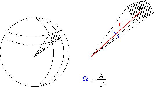
- = surface area of a sphere covered by the detector
- ie;the detectors area projected onto the surface of a sphere
- A= surface area of detector
- r=distance from interaction point to detector
- sterradians
- if your detector was a hollow ball
- sterradians

- Units
- Cross-sections have the units of Area
- 1 barn =
- [units of ] =
- Luminosity

- Fixed target scattering
- = # of particles in =
- is the area of the ring of incident particles
- = # particles in a ring of radius and thickness
You can measure if you measure the # of particles detected in a known detector solid angle from a known incident particle Flux () as
Alternatively if you have a theory which tells you which you want to test experimentally with a beam of flux then you would measure counts (particles)
- Units
- = # of particles
- or for a count rate divide both sides by time and you get beam current on the RHS
- integrate and you have the total number of counts
- Classical Scattering
- In classical scattering you get the same number of particles out that you put in (no capture, conversion,..)
- tells you how the impact parameter changes with scattering angle
Example 4: Elastic Scattering
This example is an example of classical scattering.
Our goal is to find for an elastic collision of 2 impenetrable spheres of diameter . We need to look for a relationship between the impact parameter and the scattering angle. To find this relationship, let's solve this elastic scattering problem by describing the collision using the Center of Mass (C.M.) coordinate system in terms of the reduced mass. As we shall see, by using C.M. coordinate system the 2-body collision becomes a 1-body problem. Then we will describe the motion of the reduced mass in the C.M. Frame.
 Media:SPIM_ElasCollis_Lab_CM_Frame.xfig.txt
- Variable definitions
- = impact parameter ; distance of closest approach
- = mass of incoming ball
- = mass of target ball
- = iniital velocity of incoming ball in Lab Frame
- = final velocity of in Lab Frame
- = scattering angle of in Lab frame after collision
- = iniital velocity of in C.M. Frame
- = final velocity of in C.M. Frame
- = iniital velocity of in C.M. Frame
- = final velocity of in C.M. Frame
- = scattering angle of in C.M. frame after collision
- Determining the reduced mass

- vector definitions
- = a position vector pointing to the location of
- = a position vector pointing to the location of
- = a position vector pointing to the center of mass of the two ball system
- = the magnitude of this vector is the distance between the two masses
In the C.M. reference frame the above vectors have the following relationships
solving the above equations for and and defining the reduced mass as
- reduced mass
leads to
We can use the above reduced mass relationships to construct the Lagrangian in terms of instead of and thereby reducing the problem from a 2-body problem to a 1-body problem.
- Construct the Lagrangian
The Lagrangian is defined as:
where
kinetic energy of the system
Potential energy of the system which describes the interaction
- =
- =
after substituting derivative of the expressions for and
- =
The 2-body problem is now described by a 1-body Lagrangian we need to determine which coordinate system (cartesian, spherical,..) to use to write an expression for (). Polar seems best unless there is a dependence in the azimuthal angle.
Lagranges equations of motion are given by
where represents one of the coordinate (cannonical variables).
To get the classical scattering cross section we are interested in finding an expression for the dependence of the impact parameter on the scattering angle,.
Now lets redraw the collision in terms of a reference frame fixed on (before collision its the Lab Frame but not after collision).
 Media:SPIM_ElasColls_CMFrame_xfig.txt
The C.M. Frame rides along the center of mass, the above coordinate system though has its origin on . The above drawing identifies and for the system at the point of the collision in which the CM frame is a distance (the size of the ball) from the origin of the coordinate system fixed to . If then there is no collision (), otherwise a collision happens when r=a (the distance between the balls is equal to their diameter). A head on collision is defined as ().
- Observation
- as gets smaller, gets bigger
Using plane polar coordinates () we can describe the problem in the lab frame as:
Lagranges Equation of Motion:
there is a constant of motion ( Constant angular momentum)
substitute into
The two equations above are in terms of and whereas our goal is to find an expression for . Since is related to and is related to (; see figure above) we should try and find expressions for in terms of
- Trick
- or
We now need an expression for in order to integrate the above equation to determine the functional dependence of and hence.
Since Energy is conserved (Elastic Scattering), we may define the Hamiltonian as
solving for
substituting the above into the equation for and integrating:
For :
substituting this expression for into the last expression for above :
- Integral Table
let
then
or
- Now substitute the above into the expression for
drop the negative sign, sqrt in denominator allows this, and use the trig identity
- compare with result from definition
- = scattering cross-section
- number of particles scattered = number of incident particles
- Area = = The area profile in which a collision occurs( the ball diameter is )

Lab Frame Cross Sections
The C.M. frame is often chosen to theoretically calculate cross-sections even though experiments are conducted in the Lab frame. In such cases you will need to transform cross-sections between two frames.
The total cross-section should be frame independent
or
where
is in the CM frame and is in the Lab frame.
- A non-relativistic transformation
The transformation is governed by the dependence of on
Lets return back to our picture of the scattering Process
if we superimpose the vectors and we have

Trig identities (non-relativistic Gallilean transformation) tell us
solving for
For an elastic collision only the directions change in the CM Frame: &
- From the definition of the C.M.
- conservation of momentum in CM Frame
- Gallilean Coordinate transformation
- another expression for
using the above gallilean transformation we can do the following
or
after a little trig substitution
constant
now use the chain rule to find
- constant
after substitution:
For the above equation to be more useful one would prefer to recast it in terms of only and masses.
Stopping Power
Ann. Phys. vol. 5, 325, (1930)
Bethe Equation
Classical Energy Loss
Consider the energy lost when a particle of charge () traveling at speed is scattered by a target of charge (). Assume only the coulomb force causes the particle to scatter from the target as shown below.

- Notice
- as is scattered the horizontal component of the coulomb force () flips direction; ie net horizontal force for the scattering
where
- k =
- r = distance between incident projectile and target atom
- b= impact parameter of collision
Using the definition of Impulse one can determine the momentum change of as
Let's assume that the energy lost by the incident particle is absorbed by an electron in the target atom. This energy may be cast in terms of the incident particles momentum change as
By calculating the change in momentum () of the incident particle we can infer that the energy lost by the incident particle is absorbed by one of the target material's atomic electrons.
using we have
casting this in terms of the classical atomic electron radius
- just equate
Then
and
- : = 1 here because I shall assume the energy is lost to just the electron and the Atom is a spectator
Now let's calculate an expression representing the AVERAGE energy lost for an incident particle traversing a material of some thickness.
Let
- = Probability of an interaction taking place which results in an energy loss
If we let
Z = Atomic Number = # electrons in target Atom = number of protons in an Atom
N = Avagadros number =
A = Atomic mass =
= probability of hitting an atomic electron in the area of an annulus of radius () with an energy transfer between and
Then
- = energy lost by the incident particle per distance traversed through the material
I am just adding up all the energy losses weighted by the probability of the energy loss to find the total energy loss.
- What is
- = probability of an energy transfer taking place = probability of an interaction = [ Atoms /g]
- classically
- In practice is a measured cross-section which is a function of energy.
- =
- =
- =
where if A=1
The limits of the above integral should be more physical in order to reflect the limits of the physics interaction. Let b_{min} and b_{max} represent the minimum and maximum possible impact parameter where the physics is discribed, as shown above, by the coulomb force.
- What is ?
if then diverges and the energy transfer . Physically there is a maximum energy that may be transferred before the physics of the problem changes (ie: nuclear excitation, jet production, ...). The de Borglie wavelength of the atom is used to estimate a value for such that
- What is ?
As gets bigger the interaction is "softer" and longer. If the interaction time () is so long that it is equivalent to an electron orbit () then the atom looks more like it is neutrally charged. You move from an interaction in which the electron orbit is perturbed adiabatically such that there is no orbit change and the minimum amount of energy is transferred to no interaction taking place because the atom is neutral.
Let
- : fields at high velocities get Lorentz contracted
- : I mean excitation energy of target material ( )
Condition for :
Example 5: Find for a 10 MeV proton hitting a liquid hydrogen () target
A = Z=z=1
= 0.511 MeV
I = 21.8 eV : see gray data point for Liquid From Figure 27.5 on pg 6 of PDG below.

Just need to know and
"a 10 MeV proton" Kinetic Energy (K.E.) = 10 MeV =
Proton is not relativistic
Plugging in the numbers:
- How much energy is lost after 0.3 cm?
Notice that the units for energy loss are normalized by the density of the material
= 0.07
To get the actual energy lost I need to multiply by the density. So for any given atom the energy loss will depend on the state (solid, gas, liqid) of the atom as this effects the density of the material.
- = 2.2 MeV
File:SPIM HydrogenStoppingPower.pdf Compare with Triumf Kinematics Handbook, 2nd edition, September 1987, L.G. Greeniaus
Bethe-Bloch Equation
While the classical equation above works in a limited kinematic regime, the Bethe-Bloch equation includes the corrections needed to cover most kinematic regimes for heavy particle energy loss.
where
- = Max K.E. transferable to the Target of mass in a single collision.
- = correction for electron spin and very distant collisions which deforms the electron atomic orbits each process reducing dE/dx by
- = density correction term: in the classical derivation the material is treated as just a system of atoms uniformly distributed in space. These Atoms, however, give the material polarizability which can reduce the electric field (dielectric).
GEANT 4 implementation
The GEANT4 file (version 4.8.p01)
source/processes/electromagnetic/standard/src/G4BetheBlockModel.cc
is used to calculate hadron energy loss.
line 132
where
line 143
- = density corection =
line 148
- = shell correction, corrects for the classical asumption that the atomic electron's velocity is initially zero; or the the incident particles velocity is far greater than the atomic electron's velocity.
line 154
Energy Dependence

The above curve shows the energy loss per distance traveled () as a function of the incident particles energy. There are three basic regions. At low incident energies ( < 10^5 eV) the incident particle tends to excite or even ionize the atoms in the material it is penetrating. The maximum amount of energy loss per distance traveled is defined at as the Bragg peak. The region after the Bragg peak in which the energy loss per distance traveled reaches its smallest value is refered to as the point of minimum ionizing. Minimimum ionizing particles will have incident energies corresponding to this value or larger. The characteristic of the minimum ionizing particles is that their energy loss per distance traveled is essentially constant making simulations easier until the particle's energy drops below the minimum ionizing energy level as it passes through the material.
In general the Bethe-Bloch equation breaks down at low energies (below the Bragg peak) and is a good description (to within 10%) for
- and < 26 (Iron) : a.m.u = Atomic Mass Unit
the term in the Bethe-Bloch equation dominates between the Bragg peak and the minimum ionization region.
the term and its corrections influence the dependence of as you move up in energy beyond the minimum ionization point.
Energy Straggling
While the Bethe-Bloch formula gives you a way to quantify the amount of energy a heavy charged particle loses as a function of the distance traveled, you should realize that when you calculate the total energy lost via
you are only determining the AVERAGE energy loss. In other words, Bethe-Bloch is the Astochastic process describing energy loss.
In reality the energy loss process is a stochastic process because of the statistical fluctuations which occur in the actual number of collisions which take place.
Thick Absorber
A thick absorber is one in which a large number of collisions takes place. In this situation the central limit theorem from statistics tells you that the larger number of random variables involved will result in observables which are distributed in a Gaussian manner. The Gaussian distribution is a good approximation to the binomial distribution when the number of trials is large.
Forest_ErrAna_StatDist#Binomial_with_Large_N_becomes_Gaussian
, and to a Poisson distribution when the mean is a lot larger than 1.
Forest_ErrAna_StatDist#Gaussian_approximation_to_Poisson_when
The gaussian probability function is defined as
where the Full Width at Half Max (FWHM) of the distribution =
In the case of energy loss, the variance using the Bethe-Bloch equation should be
the realitivistic variance is
for very thick absorbers see
C. Tschaler, NIM 64, (1968) 237 ; ibid, 61, (1968) 141
When simulating energy loss of heavy charged particles the Bethe-Bloch equation may be used to calculate a which can determine the average energy loss at the given kinetic energy of the particle. This average is then smeared according to a gaussian distribution of variance
Thin Absorbers
In thin absorbers the number of collisions is small preventing the use of the central limit theorem to describe the stochastic process of energy loss in terms of a Gaussian distribution. The large energy transfers that are possible cause the energy loss distribution to look like a Gaussian with a high energy tail (or foot).
The skewness of the resulting energy loss distribution is quantified as
- = lead term in Bethe Bloch equation
= density of absorbing material.
- = max energy transfered in 1 collision (headon / knock out collision)
This comes from the relativistic kinematics of an Elastic Collision.

Conservation of Momentum :
Conservation of Energy :
using conservation of E & P as well as substituting for you can show
- : cons of E
- : cons of P
solving for
(Landau Theory)
Landau assumed
- is max energy transfer
- electrons are free (energy transfer is so large you can neglect binding)
- incident particle maintains velocity (large momentum transfer from big mass to small mass) (bowling ball hits ping pong ball)
L. Landau, "On the Energy Loss of Fast Particles by Ionization", J. Phys., vol 8 (1944), pg 201
instead of a gaussian distribution Landau used
where

(Vavilou's Theory)
Vavilous paper
P.V. Vavilou, "Ionization losses of High Energy Heavy Particles", Soviet Physics JETP, vol 5 (1950? )pg 749
describe the physics for the case
The distribution function derived is shown below as well as a conceptual overlay of Vavilou's and Landau's distributions. (The in the picture should be a )
where

GEANT4's implementation
GEANT 4 uses the skewness parameter to determine if it will use a "fluctuations model" to calculate energy straggling or the gaussian model described in section 3.2.1.
kappa > 10
If
- > 10
and we have a thick absorber ( large step size) then the Gausian function in 3.2.1 is used to calculate energy straggling.
What happens is is calculated via then the actual energy loss predicted by the simulation is chosen from a Gaussian distribution to account for energy straggling such that the of this Gaussian distribution is given by:
where
- = electron density of the medium
- = charge of the incident particle
- = step size
- = cutoff kinetic energy for -electrons
tells GEANT where to put the cutoff for using the Gaussian distribution for energy straggling. This tells the simulation the low energy cutoff where Bethe-Bloch starts to fail due to ionization.
Delta-electrons
What is a - electron?
- electrons are also known as "knock -on" electrons and delta rays.
As heavy particles traverse a medium they can ionize electrons from atoms. The ejected electrons can be given enough energy to ionize as well.
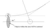
In a cloud chamber (a supercooled volume of super saturated water vapor which ionizes as charged particles pass through) such and event would look like:

The blue spiral in the above gas chamber picture is a high energy electron from the collision. The B-field is directed out of the picture.
The physics of ionization is different from the physics used to calculate Bethe-Bloch energy loss. Remember Bethe-Bloch starts to break down at low energies below the Bragg peak.
Because of this GEANT 4 sets the cutoff for this process to be
- > 1 keV
Note: The BE energies of an electron in Hydrogen is 13.6 ev and the electrons in Argon have binding energies between 15.7 eV and 3.2 keV.
Fluctuations Model: kappa < 10
If
Then GEANT 4 uses a "Fluctuations Model" to determine energy loss instead of Bethe-Bloch.
- Fluctuations Model
-
- the atom is assumed to have on 2 energy levels and
- you can excite the atom and lose either or or you can ionize the atom and lose energy according to a function .
The total energy loss in a step will be
where
- , , and are the number of collisions which are sampled from a poison distribution
- : rand = random number between 0 and 1
- = mean ionization energy
The fluctuation model was comparted with data in
K. Lassila-Perini and L. Urban, NIM, A362 (1995) pg 416
The cross sections used for excitation and ionization may be found in
H. Bichel, Rev. Mod. Phys., vol 60 (1988) pg 663
Range Straggling
- Def of Range (R)
- The distance traveled before all the particles energy is lost.
- = theoretical calculation of the path length traveled by a particle of incident energy
- Note units:
the Energy Straggling introduced in the previous section can explain why identical particles penetrate material to different depths. The energy straggling results in Range straggling.
If we do a shielding experiment where we have a source of incident particles of energy E and we count how many "punch" through a material of thickness (x) we would see a transmission coefficient which would look like

Fractional Range Straggling
fractional range straggling
Assuming the energy loss of a non-relativistic heavy ion through matter follows a Gaussian (thick absorber)
Then it can be shown that
where
- = mass of the target electrons
- = atomic mass of the Projectile
since
- kg
and
- 1 a.m.u. = kg
then
- = 1.17 % if using a proton (A=1)
The above is a "back of the envelope" estimate. The experimentally measured values for Cu, Al, and Be target using a proton projectile are

If the incident projectile is an electron then making electron range straggling a vague concept.
There are several definitions of electron range
- 1.) Maximum Range ()
- This range is defined using the continuous slowing down approximation (CSDA) in the electrons are assumed to have many collisions over very small dimensions making it appear to be continuous energy loss instead of discrete. The range is then calculated by integrating over these average energy losses .
- 2.) Practical Range ()
- This stopping distance is defined by extrapolating the electron transmission curve to zero (see below).

Electron Capture and Loss
Bohr Criterion
- "A rapidly moving nucleus is fully ionized if its velocity exceeds that of its most tightly bound electron"
The Bohr Model:
for the inner most electron ()
- Electron K.E. =
- the fine structure constant
If the nucleus is fully ionized
or
if
alternatively if the ion is moving through a material with a speed such that
Then electrons may be captured by the projectile and lost by the target.
Z-effective
Describing the charge state of your heavy ion traveling through matter at a velocity below the Bohr criterion is very complicated. There is a competition between electron capture and loss. Accurate cross sections are needed to simulate the process reliably.
Some insight into this process can be found using the Thomas-Fermi model
to describe an atom moving slow enough so it has captured many electrons but fast enough so its not neutral. In the Thomas-Fermi model the distribution of electrons in an atom is described as being uniformly distributed such that there are 2 electrons in each discrete volume of phase space( the space in which all possible states of a system are represented) defined using planks constant as .
For the purpose of simulations you would like a relationship for in terms of and .
It is usually adequate to use fits for empirical data as long as we know that we are in the kinematic range in which those fits are valid.
when MeV the data indicates that
where
- effective charge f the projectile =
- = number of protons
- = average number of captured electrons
When calculating stopping power for E < 10 MeV you use in the Bethe-Bloch equation.
Note: As the ions charge state fluctuates while it slows down (or if accelerated through materials) you will need to recalculate the energy loss, and as a result you will get larger energy loss fluctuations in this energy range.
For thin absorber you will look for stripping and loss cross sections.
- Here a thin absorber is one whose thickness is less than the charge equilibrium distance defined as the distance traveled until the projectile's velocity is
A rule of thumb is that a thin absorber for low energy ions has a thickness
For thick absorbers: The experimentally determined expression for the change in from is
Multiple Scattering
The Bethe-Bloch equation tells us how much energy is lost and GEANT4s calculation of this energy is described above.
Now we need to know which direction the scattered particle goes after it has lost this energy.
The work of Moliere describes the angular deflection of the particle which lost the energy thereby leading to a prediction of the Cross-section. GEANT4 though uses the more complete Lewis theory to describe Multiple Couloumb Scattering (MCS) sometimes generically referred to as multiple scattering.
There are 3 regions in which coulomb scattering is calculated
- 1.) Single Scattering
- For thin materials.
- If the probability of more than 1 coulomb scattering is small
- The use the Rutherford formula for
- 2.)Multiple Scattering
- In this case the number of independent scatterings is large (N > 20) and the energy loss is small such that the problem can be treated statisticaly to obtain a probability distribution for the net deflection angle as a function of the material thickness that is traversed.
- 3.) Plural Scattering
- If 1< N 20 then you can't use Rutherford to describe the scattering nor use a normal random statistical description.
see E. Keil, Z. Naturforsch, vol 15 (1960), pg 1031
Reviews of rigorous multiple scattering calculations may be found in
- P.C. Hemmer, et. al., Phys. Rev, vol 168 (1968), pg 294
GEANT4's implementation of MSC (N>20)
GEANT4 models MSC when N>20 using model functions to determine the angular and spatial distributions chosen to give the same moments of these distributions as the Lewis theory.
- H.W. Lewis, Phys. Rev., vol 78 (1950), pg 526
modern versions of the above are at
- J.M. Fernandez-Varea, et. al., NIM, B73 (1993), pg 447
- I. Kawrakow, et. al., NIM, B142 (1998) pg 253
When N>20 multiple scattering can be described as a statistical process using a modified version of the Boltzman transport equation from statistical mechanics.
- Note
- The simulation step size is chosen such that (N>20), If you have materials so thin that N < 20 then GEANT4 will likely skip the material. (one way around this is to increase the thickness and change the density). If the material thickness can't be increased because its sandwhiched between two other materials then you will need to write a special step algorithm for the volume and have GEANT4 use it for the step.
Let the distribution function for a system of incident particles traveling through a material.
where
- arc length of the particle's path through the material
- position of a charged particle
- direction of motion of the particle
The multiple scattering experienced by a single charged particle traveling through the material is then simulated by sampling from the distribution
The governing transport/diffusion equation is based on the continuity equation but with a "sink" term representing the possibility of collisions ejecting particles out of the volume.

where
- = number of atoms per volume
- = cross sections for elastic scattering per Solid angle
To solve the above diffusion equation the distribution function, is expanded in Spherical Harmonics ( ) and expand in Legendre Polynomials () since it has no angle dependence.
- Note
- For Coulomb Scattering in polar coordinates you can write the potential in terms of Legendre Polynomials such that:
- = in polar coordinates
- = (the sqrt term above is expanded using binomial series
after substituting into the diffusion equation and doing the integral on the righ hand side you get
where
- = transport mean free path for the distribution function ( symmetry is assumed making it independent)
From the above one can find the average distances traveled and the average deflection angle of the distribution. Again, see :
- J.M. Fernandez-Varea, et. al., NIM, B73 (1993), pg 447
The "moments" of are defined as
- = mean geometrical path length
Notice there are 3 lengths

- = geometrical path length between endpoints of the step =
- = true path length = actual length of the path taken by particle
- - mean geometrical path length along the z-axis
In GEANT4 the 's are taken from
If 100 eV < K.E. of electron or positron < 10 MeV
- D. Liljequist, J. Applied Phys, vol 62 (1987), 342
- J. Applied Phys, vol 68 (1990), 3061
If K.E. > 10 MeV
- R. Mogol, Atomic Data, Nucl, Data tables, vol 65 (1997) pg 55
with <z> now known GEANT will try to determine "" for the energy loss and scattering calculations.
A model is used for this where
where
- = stepsize
- at end of strep
while is calculable, GEANT4 evaluates from a probability distribution whose general form is
where
- are normalization constants
- are parameters which follow the work reported in
- V.L. Highland, NIM, vol 219 (1975) pg497
The GEANT4 files in version 4.8 were located in
/source/processes/electromagnetic/utils/src/G4VMultipleScattering.cc
and
/source/processes/electromagnetic/standard/src/G4MscModel.cc
/source/processes/electromagnetic/standard/src/G4MultipleScattering.cc
Interactions of Electrons and Photons with Matter
Bremsstrahlung
- Definition
- Radiation produced when a charged particle is deflected by the electric field of nuclei in a material.
- Note: There is also electron-electron brehmstrahlung but the interaction is with the electric field of the materials atomic electrons.
The Cross section formula is given in Formula 3Cs, pg 928 of reference H.W. Koch & J.W Motz, Rev. Mod. Phys., vol 31 (1959) pg 920 as
- Note
- Bethe & Heitler first calculated this radiation in 1934 which is why you will sometimes hear Bremsstrahlung radiation refererd to as Bethe-Heitler.
where
- = initial total energy of the electron
- = final total energy of the electron
- = energy of the emitted photon
- = Atomic number = number of protons in target material
- = charge screening parameter
Coulomb correction to using the Born approximation (approximation assumes the incident particle is a plane wave interacting with a static E-field the correction accounts for changes iin the plane wave due to the presence of the field) Charge screening and the coulomb correction are different effects that have been shown to be additive/independent. File:Haug 2008.pdf
- and = screening functions that depend on Z
if
For Z<5 see Tsai, Rev.Mod. Phys., vol 46 (1974) pg 815
- if use Equation 3.46 and 3.47
- if use Equation 3.25 and 3.26
- Note
- Energy loss via Bethe-Bloch is due to coulomb deflection and is a continuous process while Bremsstrahlung is a discrete process (emission of photons)
- We now know 2 ways charged particles can loose energy when passsing through matter.
- Energy loss
- : Bremsstrahlung
- : Bethe-Bloch (collision)
where
- = Energy of emmitted photon
- = Probabitlity of Energy loss
The quantity is defined such that
is a macroscopic function of a given material rather than just the energy which we will use to define a common property of materials known as the radiation length
where
- case is no screening and
- case has
The energy loss equation becomes
- Note
- for intermediate value of you need to integrate numerically
- : Bremsstrahlung
- : Bethe-Bloch
The illustration below shows the relative contributions of Bethe-Bloch and Bremsstrahlung to the total energy loss according to the above functional dependence. At low energies the physics of collisions dominates the loss (Bethe-Bloch) and as energy increases the discrete loss by radiation begins to dominate.

- Critical Energy
At the critical energy the two energy loss processes contribute equally to the total energy lost by a charged particle interacting with matter.
- energy at which
In the PDG
- Examples
Critical Energy E_C | |
| Material | (MeV) |
| Pb | 9.51 |
| Fe | 27.4 |
| Cu | 24.8 |
| Al | 51 |
Electron-Electron Bremsstrahlung
- Electron electron bremsstrahlung
- The radiation produced as 2 electrons pass near eachother
- is essentially the same except you have thereby adding a term and not a term
reference:pg 947 from Koch and Motz, Rev. Mod. Phys, vol 31 (1959) pg 920 File:SPIM Koch andMotz RevModPhysv31 1959pg920.pdf
as a result
- =
Most calculations ignore electron-electron Brehmsstrahung because its linear in Z and doesn;t become important until low Z where measured atomic form factors are actually used and not Form factors calulated by the Thomas-Fermi-Moliere Model (Z>4).
Coherent Bremsstrahlung
The above equations represent the physics of incoherent bremsstrahlung production.
http://137.99.79.133/halld/tagger/references/inelasticBrems-94.pdf
Radiation Length (Xo)
- Radiation Length
- The distance an electron travels through matter until loosing of its energy due to radiation .
in the high energy limit where can be ignored
or
where
- = Radiation Length of a given material
ie:
- if Then = Energy of electron after traveling a distance of through the material
Table of Radiation Lengths for several materials | |
| Material | (cm) |
| Air | 30,050 |
| Al | 8.9 |
| Cu | 1.43 |
| Fe | 1.76 |
| H2O | 36.1 |
| NaI | 2.59 |
| Pb | 0.56 |
| Polystyrene | 42.9 |
| Scintillators | 42.2 |
- If we have complete screening
- Then
- =
where
- = radiation logarithm for elastic Atomic scattering
- = radiation logarithm for inelastic Atomic scattering
- :Z < 92
- Quick Estimates
- Examples of Radiation length
- an electron has lost 1/3 of its original energy after traveling 1 radiation length (1 ) through the material
- an electron has lost 1/7 of its original energy after traveling 2 radiation lengths (2 ) through the material
- an electron has lost 1/20 of its original energy after traveling 3 radiation lengths (3 ) through the material
- After 2.3 radiation lengths the electron energy is down by a factor of 10 from its original value.
Bremsstrahlung in GEANT 4
GEANT4 uses an energy cut off to decide whether to use a continuous energy loss algorithm (msc, Bethe-Bloch, soft photons) or to generate a secondary particle (photon) and use Bremsstrahliung.
- = incident particle K.E. cutof = secondary particle production threshold
- = photon energy cutoff below which photons are treated as continuous energy loss.
- if then no photon is created and the effect of the soft photon reaction is treated as a continuous energy loss via
- = continuous energy loss via "soft" photon emission
- = cross sections parametrerized by the Evaluated Electrons Data Library (EEDL)
- reference: J. Tuli, "Evaluated Nuclear Structure Data File", BNL-NCS - 51655 -Rev 87, 1987 from Brookhaven Nat. Lab
- see National Nuclear Data Center:
- Note
- Soft photons are photons created in the scattering process which have less energy than the energy of the particles participating in the interaction. Soft photon are not energtic enough to be detected.
To improve simulation speed though, GEANT 4 actually uses a fit to the above cross sections such that
where
- = electron mass
- = kinetic energy of incident particle
- = Avagadros number
- = constants
- = polynomial (in log(T) ) chosen to fit the data
- if then a photon is created and tracked
- The energy of the emitted photon is determine by sampling a probability distribution from
- S. Seltzer and M. Berger, Atomic Data & Nucle. Data tables, vol 35 (1986) pg 345-418
and
- the angular distribution () is sampled according to
- E. Acosta, Appl. Phys. Letter, vol 80 # 17 (2002) pg 3228-3230
Note
- The MC program PENELOPE was used to generate the energy distributions that are sampled
- GEANT4 uses a modified version of base equations for bremsstrahlung with model corrections for
- LPM effect
- There is also a correction kown as the Landau Pomeranchuk Migdal (LPM) effect which corrects for multiple scattering experiences by the electron during the scattering which causes the emission of a photon.
Bragg's Rule for compound materials
The radiation length for compounds and mixtures is determined by parallel weighting (resistors in parallel)
where
- = fraction , by wieght, of each element in the mixture/compound.
- = # of atoms of element "i"
- = atomic # of element "i"
- = effective atomic mass of the compound/mixture
Photo-electric effect
The photo-electric effect identifies the physics process by which bound electrons in an atom are liberated by an interaction with an incident photon.

where
- = incident photon energy
- = electron binding energy
Moseley's Law
Moseley's law approximates the binding energies of electrons in atoms as
- (eV)
X-ray electron shells are labeled K,L,M
| Shell | n | Spect. Notation (low E) | Spect. Notation (High E) | k_s |
| K | 1 | 3 | ||
| L | 2 | 3P{3/2} | 5 |
- Example
- Binding Energies for Argon (A=18) "Chemical Rubber Company Handbook of Chemistry and Physics", CRC press. Boca Raton FL, 81st ed, 2000.
| Shell | n | Spect. Notation | Binding Energy (eV) | ||
| Measured | GEANT4 | Moseley | |||
| 1 | 3218 | 3178 | 3061 | ||
| 2 | 328 | 313.5 | 575 | ||
| 2 | 251 | 247 | 575 | ||
| 2 | 248.4 | 247 | 575 | ||
Binding energies for a few common elements
| Element | Binding Energy (eV) | ||||
| n=1 | n=2 | n=3 | |||
| B | 201 | 14.2 | 8.3 | ||
| C | 298 | 17.9 | 11.4 | ||
| N | 450 | 26 | 15 | ||
| O | 548 | 33 | 13.6 | ||
| Na | 1083 | 71 | 38 | 5.2 | |
| Mg | 1313 | 94 | 55 | 7.7 | |
| Al | 1573 | 126 | 81 | 11 | 6 |
| Si | 1854 | 157 | 107 | 15 | 8.2 |
| P | 2167 | 195 | 141 | 20 | 10.5 |
| S | 2490 | 236 | 172 | 21.3 | 10.4 |
| Cl | 2844 | 279 | 210 | 25 | 13 |
| K | 3615 | 386 | 303 | 41 | 25 |
Photo-electric cross section
- the most general expression
where
- = scattered electron wave number [ ]
- = incident photon wave frequency
- = incident photon polarization
- = momentum given to the atom divided by Plank's constant (h)
if the electron's K.E. after emission is larger than its binding energy
then
For K shell emmission
at higher energies (the ultra-relativistic limit
References
http://physics.nist.gov/PhysRefData/Xcom/html/xcom1.html
http://www-amdis.iaea.org/LANL/
http://www.nist.gov/pml/data/ionization/index.cfm
Mass Attenuation Coefficient
The mass attenuation coefficient is used to describe the attenutation of a photon interacting with matter via the photo-electric effect ( absorption), coherent scattering (Rayleigh), incoherent scattering (Compton), or pair production.
- = linear photo-electric attenutaion
- = density of the material
- Eample
- Below is an example of the mass atenuation coefficeint as a function of the incident photon energy

a 10 keV photon (0.01 MeV) will have when traveling through water
- = attenuation coefficient
- = intensity of light
- if
- = half length = = 0.69 cm
This means that 1/2 of the photons impinging on water get absorbed by the water atoms after a depth of 0.69 cm.
- Scaling
- Sometimes when is not available for your material you can scale a of a material with similar atomic number using the equation
where the coefficient varies with the photon energy from 4 5 according to:

GEANT4
GEANT4 uses a parameterization of photon absorption cross sections to determine the mean free path, atomic shell data to determine the ejected electron energy, and the k-shell angular distribution to determine the direction of the ejected electron.
The fit to the photoabsorption cross sections
- The photoabsorption cross section is parametrized according to
where
- are determined by a least squares fit to the data as outlined in
F. Biggs & R. Lighthill, Sandia Lab Preprint, SAND 87-0070 (1990)
File:Biggs Lighthill SandiaPreprint 87-0070.pdf
You select by sampling from a distribution generated by the above cross section.
The mean free path () of the photon through the material is given by
where
K.E. of ejected electron
Given that a photo-electric event happens then the energy of the ejected electron is given by
where
- = energy of the incident photon
- = electron shell energy from the closest available atomic shell as tabulated in data/G4EMLOW/fluor/binding.dat
The shell is selected according to the shell cross sections
Electron direction
The ejected electron is chosen by an angle according to the Souter-Gavrila distribution (Gavrila_M._Phys.Rev._vol113_1959_pg514) in the "standard" package such that
where rnd is a random number chosen such that
Physics Models
G4PhotoElectricEffect
This model will generate an ionized electron which is about the same as the incident photon energy. Don't use this one if your simulation is sensitive to atomic energy levels (ie; looking at keV energy effects). This should be O.K. if you are just interested in attenuating photons.
G4LowEnergyPhotoElectric
This process will generate ionized electrons for each possible electron binding energy which is less than the incident photon energy. It should be cross section weighted.
This model seems to break when 100 keV (GEANT4 version 4.8)
PAI Model
PhotoAbsorption Ionizaton (PAI) Model
The PAI model uses a least squares fit of a 4th order polynomial in to the experimental photoabsorption data for the cross section such than
where
- = fit coefficent for energy bin
- = energy transfered in the ionization collision
Compton Scattering
Compton scattering is like the photo-electric effect except the photon isn't absorbed but scattered by atomic electrons.
"Ideal" compton scattering is described in terms of free electrons.

The collision is elastic
- = electron compton wavelength =
- = electron final kinetic energy
- = ejected electron angle w.r.t original photon direction
- Note
- : No electrons can be backscattered in the compton process.
- The photon can backscattered
- = Max energy transfered to the
- = The max energy transfer point corresponds to the "compton" edge
- Example
- Find of the compton edge for a given .
- If = 8 keV
- Then eV = max energy lost by photon and given to electron

Cross Section
The Klein-Nishina formula (Oskar Klein & Yoshio Nashina, Z. fur Phys., vol 52 (1929), pg 853 ) is given as
where
- Note
- The above cross section is for a free electron. Multiple by (the number of electrons in the target) to get the atomic cross section.
After integrating over

Energy Distribution
The compton electron energy distribution can be evaluated from the differential cross section below
where
- barns
- MeV
GEANT 4
GEANT 4 parametrized the Compton cross section to reproduce the data down to 10 keV using the expression
- are determined from fit
The data used in the fit may be found in
- Hubbell, Grimm, & Overbo, J. Phys. Chem. Ref. Data 9, (1980) pg 1023
- H. Storm, Nucl. Data Tables, A7 (1970) pg 565
In addition to the default and low energy models which come with GEANT4 (as was available with the Photo Electric effect), there is also a model called "G4LECS" which may be installed.
- Models
- a.) G4ComptonScattering: listed as "compt" in the process name. No Rayleigh scattering in the model.
- b.) G4LowEnergyCompton: Process name is "LowEnCompton" in the tracking code. It has errors in the treatment of Rayleigh scattering and does not account for doppler broadening (the effect of bound electron momentum on the scattered particle energies).
- c.) G4LECS: Bound electron effects are corrected for on an :shell-by-shell" basis. Rayleigh scattering is modeled using the coherent scattering cross section and form factor data. The Doppler broadening effect is included ( a result of the compton telescope simulation work).
- Note
- Thomson & Rayleigh scattering are classical processes related to Compton scattering. Klein-Nishina formula reduces to the Thomson cross section at low energies such that . Thomson scattering produces polarized light because at these low non-relativistic energies the particle that absorbs the photon emits it in a direction perpendicular to its motion, that motion is the results of sees the oscillating E & M wave from the incident photon. Rayleigh scattering (why our sky is blue) is photon scattering from an atom as a whole, coherent scattering. No energy is transfered to the Medium in either case, only changes direction. Rayleigh scattering is the elastic scattering of the photon from a particle that is smaller than the wavelength of the light. Mei theory is used to describe elastic scattering from particles that are larger than the wavelength of the incident photon.
Pair Production
Pair production is similar to the Bremsstrahlung process.
Remember, in Bremsstrahlung the incident charged particle interacts with the of the Nucleus (or shell electron)

In pair production a photon interacts with the of the Nucleus.

when the recoil of the atom is taken into account
- = Threshold energy for pair production from an atom of mass
- Note
- You can also have photon-electron pair production analogous to electron-electron bremsstrahlung production.
Pair Production Cross Section
The pair production cross section is given by Equation 6.35 in (Bethe, Phys. Rev., vol. 93 (1964) pg 768)
at small angles
A version which assumes small angles is given in Eq 7.35 of the same reference as the triple differential cross section:
where
- photon momentum/energy
- = scattering angle of
- = scattering angle of
- angle between the and pair
- = Energy of the positron
- = Energy of the electron
- Note
- The above equations for the differential cross section are using "natural" units where
Davies' version integrates over all angles
Davies published a version which has been integrated over angles and includes some screening effects ( see Eq 35):
where
If you integrate over all positron ( ) energies you get Eq. 44 (no screening)
and Eq. 45 (complete screening)
Davies expressions were shown to work well at high energies ( MeV)
Overbo's low energy Cross sections
At low energies ( MeV), Overbo published an exact calculation in the case that the Atomic field is unscreened. Overbo then provided a fit to the results of his calculation which he claims is valid to within 0.1% for the energy range . The fit is given in Eq. 7.1 of his paper as
where
- Low Energy unscreened Born approximation total cross section for pair production
- = incident photon energy in units of the electron rest mass energy
Intermediate Energy Cross sections
For the Gradstein semi-ephirical formula is used from G. White Gradstein, Natl. Bur. Standard., Circ 583 (1957) pg 1.
where
- = empirical constant = 4.02 barns for Pb
- = empirical constant = 16.8 barns for Pb
- = Simulations_of_Particle_Interactions_with_Matter#Bremsstrahlung Bethe-Heitler cross section
Triplet production
- Triplet Production
- identifies photon-electron pair production. The recoiling electron track adds to the two tracks making three total particle tracks (kind of like pair production ionization).
A description for how to calculate the cross section for this process is illustrated for 1 in L.E. Wright, Phys. Rev. C 36 (1987) pg 582. Unfortunately, analytic expression is not given but one could construct tables of and in equation 65 of L.E. Wright's paper.
An example for may be found in Sud & Vargus, Phys. Rev. A49 (1994) pg 4624.
GEANT4 Pair production
GEANT4 uses the pair production cross section given in Tsai, Rev. Mod. Phys, vol 46 (1974) pg 815.
where
- energy of incident photon
- KE of create electron
- fraction of taken away by
- triplet production correction
- high energy coulomb correction from Davies above
- & = electron screening functions
The formula GEANT4 uses may also be found on pg 541 in J. Bono , Radiation Physics Chemistry, vol 44 (1994) pg 531
where
- = low energy coulomb correction
- = screening radius (adjustable parameter)
- = Compton wavelength
An older simulation description with graphs of the cross-sections may be found below.
File:Bigg Lighthill conversion 1Mev-100MeV SandiaPreprint SC-RR-68-619.pdf
Below is the review of Modern Physics article basically summarizing all of the physics for pair production up to 1969
File:RevModPhys PairPoduction 1969 MotzOlsonKoch.pdf
Contributions as function of Z
The plot below shows the contributions of the three photon absorption physics processes as a function of the incident photon energy and the Z of the target material. At low energy (keV), the photo-electric effect dominant while at high energies (> 1 MeV) pair production starts to dominate. Compton scattering dominates in the intermediate energy region.

Hadronic Interactions
Proton Bremsstrahlung
- = cross section for dipole radiation emitted at 90 degrees with respect to incident beam of particles scattered in a Coulomb field.
File:ProtonBrem Drell Huang PhysRev v99 n3 1955 pg686.pdf
Pluto event generator
A ROOT based Hadronic Simulation package based on Pluto
I installed Pluto V 5.14.1 on inca
I needed to set the environmental variables under tcsh
setenv ROOTSYS ~/src/ROOT/root
setenv PATH ${PATH}:${ROOTSYS}/bin
setenv LD_LIBRARY_PATH $ROOTSYS/lib
There is a subdirectory called "macros"
cd macros
Go to that subdirectory and type root, this will run the contents of the file "rootlogin.C"
cd macros
inca:~/src/Pluto/pluto_v5.14.1/macros> root
 *******************************************
 *                                         *
 *        W E L C O M E  to  R O O T       *
 *                                         *
 *   Version   5.17/03    30 August 2007   *
 *                                         *
 *  You are welcome to visit our Web site  *
 *          http://root.cern.ch            *
 *                                         *
 *******************************************
Compiled on 5 September 2007 for linux with thread support.
CINT/ROOT C/C++ Interpreter version 5.16.24, July 26, 2007
Type ? for help. Commands must be C++ statements.
Enclose multiple statements between { }.
 *********************************************************
 * The Pluto event generator
 * (C) HADES collaboration and all contributing AUTHORS
 * www-hades.gsi.de/computing/pluto/html/PlutoIndex.html
 * Version: 5.14.1
 * Compiled on 10 December 2008
 *********************************************************
Shared library Pluto.so loaded
to run a pp elastic model type
root [0] .x pp_elastic.C
a root ntuple is generate called "pp_elastic.root"
you can then analyze the data in the root file with
data->MakeClass();
the above command within root generates an analysis skeleton program.
using t.Show you can see the structure of the events within the ntuple. A few functions are also stored in the root tree which you can use. You can use the root file event to create an input file which GEANT4 can then use as its event generator. GEANT4 then reads the events in and propagates them through your geometry.
Neutron Interactions
| Name | Energy |
| Cold Neutron | micro eV |
| Thermal | eV |
| epithermal | |
| fast | |
| high energy |
Note: Interaction length for neutrons is ~ .
Neutrons are even better than photons for penetrating matter.
Elastic scattering
File:Elastic scattering from Nuclei.jpg
velocity of CM frame
Magnitude of Neutron velocity in CM frame before and after collision
Magnitude of Nucleus velocity in CM frame before and after collision
Note: In elastic collision only the particles direction changes.
where
After substitution we get following:
when , .
Minimum energy of scattered Neutron in LAB frame.
After substituting
Note:
Energy of recoil Nuclei in CM frame.
Conservation of Energy:
Inelastic Scattering
Homework Problems
HomeWork_Simulations_of_Particle_Interactions_with_Matter
Resources
Building GEANT4.9.5