Simulations of Particle Interactions with Matter

Overview

Particle Detection

A device detects a particle only after the particle transfers energy to the device.

Energy intrinsic to a device depends on the material used in a device

Some device of material with an average atomic number ([math]Z[/math]) is at some temperature ([math]T[/math]). The materials atoms are in constant thermal motion (unless T = zero degrees Klevin).

Statistical Thermodynamics tells us that the canonical energy distribution of the atoms is given by the Maxwell-Boltzmann statistics such that

[math]P(E) = \frac{1}{kT} e^{-\frac{E}{kT}}[/math]

[math]P(E)[/math] represents the probability of any atom in the system having an energy [math]E[/math] where

[math]k= 1.38 \times 10^{-23} \frac{J}{mole \cdot K}[/math]

Note: You may be more familiar with the Maxwell-Boltzmann distribution in the form

[math]N(\nu) = 4 \pi N \left ( \frac{m}{2\pi k T} \right ) ^{3/2} v^2 e^{-mv^2/2kT}[/math]

where [math]N(v) \Delta v[/math] would represent the molesules in the gas sample with speeds between [math]v[/math] and [math]v + \Delta v[/math]

Example 1: P(E=5 eV)

What is the probability that an atom in a 12.011 gram block of carbon would have and energy of 5 eV?

First lets check that the probability distribution is Normailized; ie: does [math]\int_0^{\infty} P(E) dE =1[/math]?

[math]\int_0^{\infty} P(E) dE = \int_0^{\infty} \frac{1}{kT} e^{-\frac{E}{kT}} dE = \frac{1}{kT} \frac{1}{\frac{1}{-kT}} e^{-\frac{E}{kT}} \mid_0^{\infty} = - [e^{-\infty} - e^0]= 1[/math]

[math]P(E=5eV)[/math] is calculated by integrating P(E) over some energy interval ( ie:[math] N(v) dv[/math]). I will arbitrarily choose 4.9 eV to 5.1 eV as a starting point.

[math]\int_{4.9 eV}^{5.1 eV} P(E) dE = - [e^{-5.1 eV/kT} - e^{4.9 eV/kT}][/math]

[math]k= (1.38 \times 10^{-23} \frac{J}{mole \cdot K} ) = (1.38 \times 10^{-23} \frac{J}{mole \cdot K} )(6.42 \times 10^{18} \frac{eV}{J})= 8.614 \times 10^{-5} \frac {eV}{mole \cdot K}[/math]

assuming a room empterature of [math]T=300 K[/math]

then[math]kT = 0.0258 \frac{eV}{mole}[/math]

and

[math]\int_{4.9 eV}^{5.1 eV} P(E) dE = - [e^{-5.1/0.0258} - e^{4.9/0.0258}] = 4.48 \times 10^{-83} - 1.9 \times 10^{-86} \approx 4.48 \times 10^{-83}[/math]

or in other words the precise mathematical calculation of the probability may be approximated by just using the distribution function alone

[math]P(E=5eV) = e^{-5/0.0258} \approx 10^{-85}[/math]

This approximation breaks down as [math]E \rightarrow 0.0258 eV[/math]

Since we have 12.011 grams of carbon and 1 mole of carbon = 12.011 g = [math]6 \times 10^{23} [/math]carbon atoms

We do not expect to see a 5 eV carbon atom in a sample size of [math]6 \times 10^{23} [/math] carbon atoms when the probability of observing such an atom is [math]\approx 10^{-85}[/math]

The energy we expect to see would be calculated by

[math]\lt E\gt = \int_{0}^{\infty} E \cdot P(E) dE[/math]

If you used this block of carbon as a detector you would easily notice an event in which a carbon atom absorbed 5 eV of energy as compared to the energy of a typical atom in the carbon block.

---

Silicon detectors and Ionization chambers are two commonly used devices for detecting radiation.

approximately 1 eV of energy is all that you need to create an electron-ion pair in Silicon

[math]P(E=1 eV) = e^{-1/0.0258} \approx 10^{-17}[/math]

approximately 10 eV of energy is needed to ionize an atom in a gas chamber

[math]P(E=10 eV) = e^{-10/0.0258} \approx 10^{-169}[/math]

The low probability of having an atom with 10 eV of energy means that an ionization chamber would have a better Signal to Noise ratio (SNR) for detecting 10 eV radiation than a silicon detector

But if you cool the silicon detector to 200 degrees Kelvin (200 K) then

[math]P(E=1 eV) = e^{-1/0.0172} \approx 10^{-26} \lt \lt 10^{-17}[/math]

So cooling your detector will slow the atoms down making it more noticable when one of the atoms absorbs energy.

also, if the radiation flux is large, more electron-hole pairs are created and you get a more noticeable signal.

Unfortunately, with some detectore, like silicon, you can cause radiation damage that diminishes it's quantum efficiency for absorbing energy.

The Monte Carlo method

Stochastic

from the greek word "stachos"

a means of, relating to, or characterized by conjecture and randomness.

A stochastic process is one whose behavior is non-deterministic in that the next state of the process is partially determined.

Physics has many such non-deterministic systems:

• Quantum Mechanics
• Thermodynamics

Basically the monte-carlo method uses a random number generator (RNG) to generate a distribution (gaussian, uniform, Poission,...) which is used to solve a stochastic process based on an astochastic description.

Example 2 Calculation of [math]\pi[/math]

Astochastic description

[math]\pi[/math] may be measured as the ratio of the area of a circle of radius [math]r[/math] divided by the area of a square of length [math]2r[/math]

File:PI from AreaRatio.jpg[math]\frac{A_{circle}}{A_{square}} = \frac{\pi r^2}{4r^2} = \frac{\pi}{4}[/math]

You can measure the value of [math]\pi[/math] if you physically measure the above ratios.

Stochastic description

Construct a dart board representing the above geometry, throw several darts at it, and look at a ratio of the number of darts in the circle to the total number of darts thrown (assuming you always hit the dart board).

Monte-Carlo Method

Here is an outline of a program to calulate [math]\pi[/math] using the Monte-Carlo method with the above Stochastic description

begin loop
 x=rnd
 y=rnd
 dist=sqrt(x*x+y*y)
 if dist <= 1.0 then numbCircHits+=1.0
 numbSquareHist += 1.0
end loop
 print PI = 4*numbCircHits/numbSquareHits

A Unix Primer

To get our feet wet using the UNIX operating system, we will try to solve example 2 above using a RNG under UNIX

List of important Commands

1. ls
2. pwd
3. cd
4. df
5. ssh
6. scp
7. mkdir
8. printenv
9. emacs, vi, vim
10. make, gcc
11. man
12. less
13. rm

---

Most of the commands executed within a shell under UNIX have command line arguments (switches) which tell the command to print information about using the command to the screen. The common forms of these switches are "-h", "--h", or "--help"

ls --help
ssh -h

the switch deponds on your flavor of UNIX

if using the switch doesn;t help you can try the "man" (sort for manual) pages (if they were installed). Try

man -k pwd

the above command will search the manual for the key word "pwd"

Example 3: using UNIX

Step

1. login to inca.
   click here for a description of logging in if using windows
2. mkdir src
3. cd src
4. cp -R ~tforest/NucSim/Day1 ./
5. ls
6. cd Day1
7. make
8. ./rndtest

Here is a web link to the source files you can copy in case the above doesn't work

Cross Sections

Definitions

Total cross section

[math]\sigma[/math] = [math]\equiv \frac{\# particles\; scattered} {\frac{ \# incident \; particles}{Area}}[/math]

Differential cross section

[math]\sigma(\theta)[/math] = [math] \frac{d \sigma}{d \Omega} \equiv \frac{\frac{\# particles\; scattered}{solid \; angle}} {\frac{ \# incident \; particles}{Area}}[/math]

Solid Angle

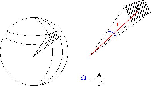
[math]\Omega[/math]= surface area of a sphere covered by the detector

ie;the detectors area projected onto the surface of a sphere

A= surface area of detector

r=distance from interaction point to detector

[math]\Omega = \frac{A}{r^2} [/math]sterradians

[math]A_{sphere} = 4 \pi r^2[/math] if your detector was a hollow ball

[math]\Omega_{max} = \frac{4 \pi r^2}{r^2} = 4\pi[/math]sterradians

Units

Cross-sections have the units of Area

1 barn = [math]10^{-28} m^2[/math]

[units of [math]\sigma(\theta)[/math]] =[math]\frac{\frac{[particles]}{[sterradian]}} {\frac{ [ particles]}{[m^2]}} = m^2[/math]

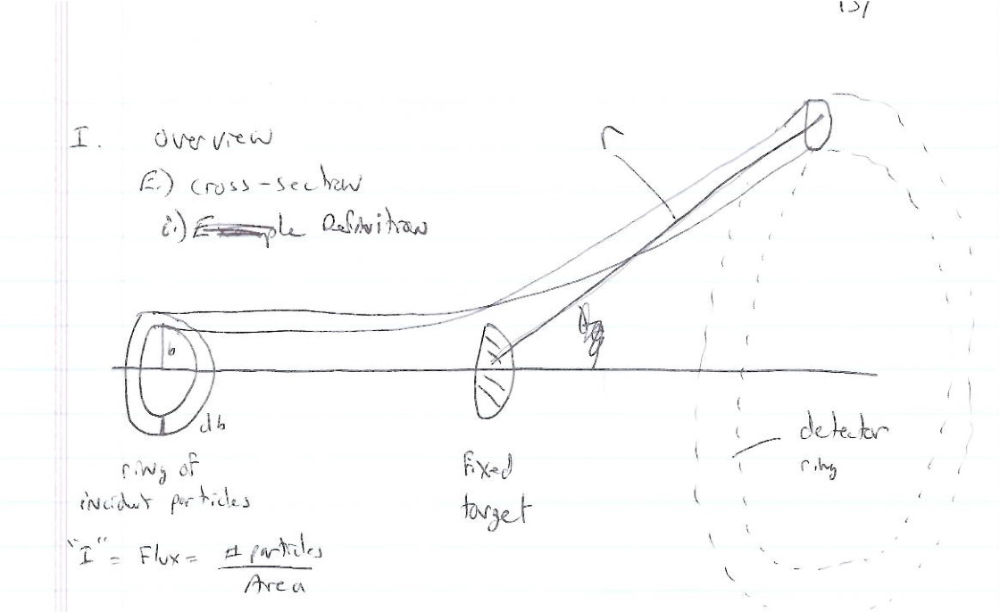
Fixed target scattering

[math]N_{in}[/math]= # of particles in = [math]I \cdot A_{in}[/math]

[math]A_{in}[/math] is the area of the ring of incident particles

[math]dN_{in} = I \cdot dA = I (2\pi b) db[/math]= # particles in a ring of radius [math]b[/math] and thickness [math]db[/math]

You can measure [math]\sigma(\theta)[/math] if you measure the # of particles detected [math]d N[/math] in a known detector solid angle [math]d \Omega[/math] from a known incident particle Flux ([math]I[/math]) as

[math]\sigma(\theta) = \frac{\frac{d N}{ d \Omega}}{I}[/math]

Alternatively if you have a theory which tells you [math]\sigma(\theta)[/math] which you want to test experimentally with a beam of flux [math]I[/math] then you would measure counts (particles)

[math]dN = I \sigma(\theta) d \Omega = I \sigma(\theta) \frac{d A}{r^2} = I \sigma(\theta) \frac{r^2 \sin(\theta) d \theta d \phi}{r^2}[/math]

Units

[math][d N] = [\frac {particles}{m^2}][m^2] [sterradian] [/math] = # of particles

or for a count rate divide both sides by time and you get beam current on the RHS

integrate and you have the total number of counts

Classical Scattering

In classical scattering you get the same number of particle out that you put in (no capture, conversion,..)

[math]d N_{in} = dN[/math]

[math]d N_{in} = I dA = I (2\pi b) db[/math]

[math]d N = I \sigma(\theta) d \Omega = I \sigma(\theta) \sin(\theta) d \theta d \phi = I \sigma(\theta) \sin(\theta) d \theta (2 \pi )[/math]

[math] I (2\pi b) db = I \sigma(\theta) \sin(\theta) d \theta (2 \pi )[/math]

[math] b db = \sigma(\theta) \sin(\theta) d \theta [/math]

[math]\sigma(\theta) = \frac{b}{\sin(\theta)}\frac{db}{d \theta}[/math]

[math]\frac{db}{d \theta}[/math] tells you how the impact parameter [math]b[/math] changes with scattering angle [math]\theta[/math]

Example 4: Elastic Scattering

This example is an example of classical scattering.

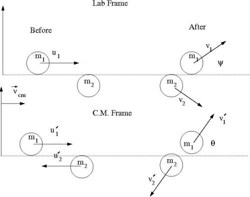
Our goal is to find [math]\sigma(\theta)[/math] for an elastic collision of 2 impenetrable spheres of diameter [math]a[/math]. To solve this elastic scattering problem we will describe the collision using the Center of Mas (C.M.) coordinate system in terms of the reduced mass. As we shall see, by using C.M. coordinate system the 2-body collision becomes a 1-body problem. Then we will describe the motion of the reduced mass in the C.M. Frame.

Media:SPIM_ElasCollis_Lab_CM_Frame.xfig.txt

Variable definitions

[math]b[/math]= impact parameter ; distance of closest approach

[math]m_1[/math]= mass of incoming ball

[math]m_2[/math]= mass of target ball

[math]u_1[/math]= iniital velocity of incoming ball in Lab Frame

[math]v_1[/math]= final velocity of [math]m_1[/math] in Lab Frame

[math]\psi[/math]= scattering angle of [math]m_1[/math] in Lab frame after collision

[math]u_1^{\prime}[/math]= iniital velocity of [math]m_1[/math] in C.M. Frame

[math]v_1^{\prime}[/math]= final velocity of [math]m_1[/math] in C.M. Frame

[math]u_2^{\prime}[/math]= iniital velocity of [math]m_2[/math] in C.M. Frame

[math]v_2^{\prime}[/math]= final velocity of [math]m_2[/math] in C.M. Frame

[math]\theta[/math]= scattering angle of [math]m_1[/math] in C.M. frame after collision

Determining the reduced mass

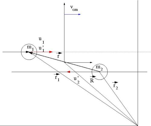
vector definitions

[math]\vec{r}_1[/math] = a position vector pointing to the location of [math]m_1[/math]

[math]\vec{r}_2[/math] = a position vector pointing to the location of [math]m_2[/math]

[math]\vec{R}[/math] = a position vector pointing to the center of mass of the two ball system

[math]\vec{r} \equiv \vec{r}_1 - \vec{r}_2[/math] = the magnitude of this vector is the distance between the two masses

In the C.M. reference frame the above vectors have the following relationships

1. [math]\vec{R} = 0 = \frac{m_1 \vec{r}_1 + m_2 \vec{r}_2}{m_1 + m_2} \Rightarrow m_2 \vec{r}_1 = -m_2 \vec{r}_2[/math]
2. [math]\vec{r}_1 - \vec{r}_2 = \vec{r}[/math]

solving the above equations for [math]\vec{r_1}[/math] and [math]\vec{r_2}[/math] and defining the reduced mass [math]\mu[/math] as

[math]\mu = \frac{m_1 \cdot m_2}{m_1 + m_2} \equiv[/math] reduced mass

leads to

[math]\vec{r}_1 = \frac{\mu}{m_1} \vec{r}[/math]

[math]\vec{r}_2 = \frac{\mu}{m_2} \vec{r}[/math]

We can use the above reduced mass relationships to construct the Lagrangian in terms of [math]\vec{r}[/math] instead of [math]\vec{r}_1[/math] and [math] \vec{r}_2[/math] thereby reducing the problem from a 2-body problem to a 1-body problem.

Construct the Lagrangian

The Lagrangian is defined as:

[math]\mathcal{L} = T - U[/math]

where

[math]T \equiv[/math] kinetic energy of the system

[math]U \equiv[/math] Potential energy of the system which describes the interaction

[math]\mathcal{L} = \frac{1}{2} |\vec{\dot{r}}_1|^2 + \frac{1}{2} |\vec{\dot{r}}_2|^2 - U[/math]

= [math]\frac{1}{2} m_1 \left (\frac{m_2}{m1+m_2} \right )^2 |\vec{\dot{r}}|^2 + \frac{1}{2} m_2 \left (\frac{m_1}{m1+m_2} \right )^2 |\vec{\dot{r}}|^2 -U(\vec{r})[/math]

after substituting derivative of the expressions for [math]\vec{r_1}[/math] and [math]\vec{r}_2[/math]

= [math]\frac{1}{2} \mu |\vec{\dot{r}}|^2 -U(\vec{r})[/math] The 2-body problem is now described by a 1-body Lagrangian

Lagranges equations of motion are given by

[math]\frac{\partial \mathcal{L}}{\partial q} = \frac{d}{dt} \frac{\partial \mathcal{L}}{\dot{q}}[/math]

where [math]q[/math] represents on of the coordinate (cannonical variables).

To get the classical scattering cross section we are interested in finding an expression for the dependence of the impact parameter on the scattering angle,[math]\frac{d b}{d \theta}[/math].

Now lets redraw the collision in terms of a reference frame fixed on [math]m_2[/math] (before collision its the Lab Frame but not after collision).

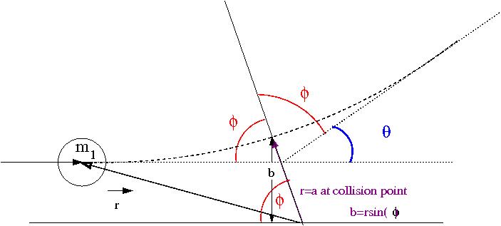Media:SPIM_ElasColls_CMFrame_xfig.txt

The C.M. Frame rides along the center of mass, the above coordinate system though has its origin on [math]m_2[/math] and only overlaps in space with the CM frame at the collision point sufficiently to illustrate [math]\theta[/math]. If [math]b \gt a[/math] then there is no collision ([math]\theta=0[/math]), otherwise a collision happens when r=a (the distance between the balls is equal to their diameter). A head on collision is defined as [math]b=0[/math] ([math]\theta=\pi[/math]).

Observation

as [math]\theta[/math] gets smaller, [math]b[/math] gets bigger

[math]\frac{d b}{d \theta} \lt 0[/math]

Using plane polar coordinates ([math]r, \phi[/math]) we can describe the problem in the lab frame as:

[math]\vec{v} = \dot{R} \hat{e}_r + r \dot{\phi} \hat{e}_{\phi}[/math]

[math]T = \frac{1}{2} \mu ( \dot{r)}^2 + r^2 \dot{\phi}^2)[/math]

[math]U(r) = \left \{ {0 \; r \gt a \atop \infty \; r \le a} \right .[/math]

[math]\mathcal{L} = T -U = \frac{1}{2} \mu ( \dot{r}^2 + r^2 \dot{\phi}^2) - U(r)[/math]

Lagranges Equation of Motion:

[math]\frac{\partial \mathcal {L}}{\partial \phi} = \frac{d}{d t} \frac{\partial \mathcal{L}}{\partial \dot{\phi}}[/math] [math]0 = \frac{d}{d t} [ \mu r^2 \dot{\phi}] \Rightarrow[/math] there is a constant of motion ( Constant angular momentum)

[math]\ell \equiv \mu r^2 \dot{\phi} = \vec{r} \times \vec{p} = \vec{r} \times \mu \vec{v} = r^2 \mu \dot{\phi}[/math]

substitute [math]\ell[/math] into [math]\mathcal{L}[/math]

[math]\mathcal{L} = \frac{1}{2} ( \mu \dot{r}^2 + \frac{\ell}{\mu r^2} ) - U(r)[/math]

The two equations above are in terms of [math]r[/math] and [math]\phi[/math] whereas our goal is to find an expression for [math]\frac{ d b}{ d \theta}[/math]. Since [math]r[/math] is related to [math]b[/math] and [math]\phi[/math] is related to[math] \theta[/math] ([math]\theta = \pi - 2\phi[/math]; see figure above) we should try and find expressions for [math]d \phi[/math] in terms of [math]r(b)[/math]

Trick

[math]\dot{\phi} = \frac{d \phi}{d t} = \frac{d \phi}{d r} \frac{d r}{d t}[/math]

[math]\Rightarrow \ell = \mu r^2 \frac{d \phi}{d r} \dot{r}[/math]

or

[math]d \phi = \frac{\ell}{\mu r^2 \dot{r}} dr[/math]

We now need an expression for [math]\dot{r}[/math] in order to integrate the above equation to determine the functional dependence of [math]\phi[/math] and hence[math] \theta[/math].

Since Energy is conserved (Elastic Scattering), we may define the Hamiltonian as

[math]H = T + U = \frac{1}{2} (mu \dot{r}^2 + \frac{\ell}{\mu r^2}) + U(r) = constant \equiv E[/math]

solving for [math]\dot{r}[/math]

[math]\dot{r} = \pm \sqrt{\frac{2(E-U(r))}{\mu} - \frac{\ell^2}{\mu^2 r^2}}[/math]

substituting the above into the equation for [math]d \phi[/math] and integrating:

[math]\phi = \int d \phi = \int_{r_{min}}^{r_{max}} \frac{\ell}{\mu r^2 \dot{R}} dr[/math]

[math]r_{min} = a \; \; \; r_{max}= \infty \; \; \; U(r) = 0 : a \le r \le \infty[/math]

[math]\phi = \int_a^{\infty} \frac{\ell} {r^2 \sqrt{2 \mu E - \frac{\ell^2}{r^2}} }dr[/math]

For [math]a \le r \le \infty[/math] : [math]E = \frac{1}{2} \mu v^2_{cm} \Rightarrow v_{cm} = \sqrt{\frac{2E}{\mu}}[/math]

[math]\vec{\ell} = \vec{r} \times \vec{p} \Rightarrow |\vec{\ell}| = |\vec{r}| |\vec{p}| \sin(\phi) = r \mu v_{cm} \sin(\phi) = r \mu \left ( \sqrt{\frac{2E}{\mu}} \right) \sin(\phi) = \sqrt{2 \mu E} r\sin(\phi) =\sqrt{2 \mu E} b[/math]

substituting this expression for [math]\ell[/math] into the last expression for [math]\phi[/math] above :

[math]\phi =\int_a^{\infty} \frac{b dr}{r\sqrt{(r^2-b^2)}}[/math]

Integral Table

[math]\int \frac{dx}{x\sqrt{(\alpha x^2+\beta x+\gamma)}} = \frac{-1}{\sqrt{-\gamma}} \sin^{-1} \left (\frac{\beta x+2\gamma}{|x|\sqrt{\beta^2-4\alpha \gamma}} \right )[/math]

let [math]x=r \;\; \alpha=1 \;\; \beta=0 \;\; \gamma=-b^2[/math]

then

[math]\phi = \left . b \frac{1}{\sqrt{-(-b^2)}} \sin^{-1} \left (\frac{-2b^2}{r\sqrt{0-4(1)(-b^2) } }\right ) \right |_a^{\infty} = \sin^{-1} (0)- \sin^{-1}(-\frac{b}{a})[/math]

or

[math]\sin(\phi) = \frac{b}{a} = \sin \left ( \frac{\pi}{2} - \frac{\theta}{2} \right ) = \cos \left ( \frac{\theta}{2} \right )[/math]

[math]\Rightarrow b = a \cos \left( \frac{\theta}{2} \right)[/math]

Now substitue the above into the expression for [math]\sigma(\theta)[/math]

[math]\sigma(\theta) = \frac{b}{\sin(\theta)} \frac{d b}{d \theta} = \frac{a \cos(\theta/2)}{sin(\theta)} a[-\sin(\theta/2)]\frac{1}{2} = \frac{a^2}{2} \frac{\cos(\theta/2) \sin(\theta/2)}{\sin(\theta)}[/math]

drop the negative sign, sqrt in denominator allows this, and use the trig identity

[math]\sin \left (\frac{\theta}{2} + \frac{\theta}{2} \right ) = \cos \left (\frac{\theta}{2} \right) \sin \left (\frac{\theta}{2} \right ) + \cos \left ( \frac{\theta}{2} \right ) \sin \left (\frac{\theta}{2} \right )[/math]

[math]\sin(\theta) = 2 \cos \left (\frac{\theta}{2} \right ) \sin \left (\frac{\theta}{2} \right )[/math]

[math]\sigma(\theta) = \frac{a^2}{2} \frac{1}{2} = \frac{a^2}{4}[/math]

[math]\sigma = \int \sigma(\theta) d \Omega = \frac{a^2}{2} \frac{1}{2} 4 \pi = \pi a^2[/math]

compare with result from definition

[math]\sigma[/math] = scattering cross-section [math]\equiv \frac{\# particles\; scattered} {\frac{ \# incident \; particles}{Area}}[/math]

number of particles scattered = number of incident particles

Area = [math] \pi a^2[/math] = The area profile in which a collision occurs

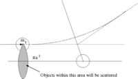
[math]\sigma = \frac{{N}}{\frac{ N}{\pi a^2}} = \pi a^2[/math]

Lab Frame Cross Sections

The C.M. frame is often chosen to theoretically calculate cross-sections even though experiments are conducted in the Lab frame. In such cases you will need to transform cross-sections between two frames.

The total cross-section should be frame independent

[math]\sigma_{C.M.} = \sigma_{Lab}[/math]

or

[math]\sigma(\theta) d \Omega = \sigma(\psi) d \Omega^{\prime}[/math]

where

[math]\theta[/math] is in the CM frame and [math]\psi[/math] is in the Lab frame.

A non-relativistic transformation

[math]\sigma(\theta) d \Omega = \sigma(\psi) d \Omega^{\prime}[/math]

[math]\sigma(\theta) 2 \pi \sin(\theta) d \theta = \sigma(\psi) 2 \pi \sin (\psi) d \psi[/math]

[math]\Rightarrow \sigma(\psi) = \frac{\sin(\theta)}{\sin(\psi)} \frac{d \theta}{d \psi} \sigma(\theta)[/math]

The transformation is governed by the dependence of [math]\theta[/math] on [math] \psi[/math] [math] \left( \frac{d \theta}{d \psi} \right )[/math]

Lets return back to our picture of the scattering Process

if we superimpose the vectors [math]\vec{v}_1[/math] and [math]\vec{v}_1^{\prime}[/math] we have

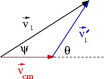
Trig identities (non-relativistic Gallilean transformation) tell us

[math]v_1 \sin(\psi) = v_1^{\prime} \sin(\theta)[/math]

[math]v_1 cos(\psi) = v_{cm} + v_1^{\prime} \cos(\theta)[/math]

solving for [math]\psi[/math]

[math]\tan(\psi) = \frac{\sin(\psi)}{\cos(\psi)} = \frac{v_1^{\prime} \sin(\theta)/v_1}{\frac{v_{CM}}{v_1} + \frac{v_1^{\prime} \cos(\theta)}{v_1} } = \frac{\sin(\theta)}{\cos(\theta) + \frac{v_{CM}}{v_1^{\prime}}}[/math]

For an elastic collision only the directions change in the CM Frame: [math]u_1^{\prime}= v_1^{\prime}[/math] & [math]u_1^{\prime}= v_2^{\prime}[/math]

From the definition of the C.M.

[math]\vec{v}_{CM} = \frac{m_1 \vec{u}_1 + m_2 \vec{u}_2}{m_1+m_2} = \frac{m_1}{m_1+m_2} \vec{u}_1[/math]

conservation of momentum in CM Frame [math]\Rightarrow[/math]

[math]m_1 u_1^{\prime} = - m_2 u_2{\prime}[/math]

[math] \Rightarrow v_1^{\prime} = u_1^{\prime} = \frac{-m_2}{m_1} u_2^{\prime}[/math]

Gallilean Coordinate transformation

[math]\vec{u}_1 = \vec{u}_1^{\prime} + \vec{v}_{CM} = \vec{u}_1^{\prime} + \frac{m_1}{m_1+m_2} \vec{u}_1[/math]

[math]\Rightarrow u_1{\prime} = \left [ 1 - \frac{m_1}{m_1 + m_2} \right ] u_1 = \frac{m_2}{m_1+m_2}u_1[/math]

[math]\Rightarrow v_1^{\prime} = u_1^{\prime} =\frac{m_2}{m_1+m_2} u_1[/math]

another experission for [math]\psi[/math]

using the above gallilean transformation we can do the following

[math]\frac{v_{CM}}{v_1^{\prime}}= \frac{\frac{m_1}{m_1+m_2} u_1}{\frac{m_2}{m_1+m_2} u_1} = \frac{m_1}{m_2}[/math]

or

[math]\tan(\psi) = \frac{\sin(\theta)}{\cos(\theta) + \frac{m_1}{m_2}}[/math]

after a little trig substitution

[math]\Rightarrow \frac{m_1}{m_2} = \frac{sin(\theta - \psi)}{\sin(\psi)} =[/math] constant

now use the chain rule to find [math]\frac{d \theta}{d \psi}[/math]

[math]f \equiv \frac{sin(\theta - \psi)}{\sin(\psi)} =[/math] constant

[math]df = 0 = \frac{ \partial f}{\partial \psi} d \psi + \frac{ \partial f}{\partial \theta} d \theta [/math]

[math]\Rightarrow \frac{d \theta}{d \psi} = \frac{-\frac{ \partial f}{\partial \psi} }{\frac{ \partial f}{\partial \theta} }[/math]

[math]-\frac{ \partial f}{\partial \psi} = \frac{\cos(\theta - \psi)}{\sin(\psi)} + \frac{\sin(\theta - \psi)}{\sin(\psi)}[/math]

[math]\frac{ \partial f}{\partial \theta }= 1 + \frac{\sin(\theta - \psi) \cos(\psi)}{\cos(\theta - \psi) \sin(\psi)}[/math]

after substitution:

[math]\sigma(\psi) = \frac{\sin(\theta)}{\sin(\psi)} \frac{d \theta}{d \psi} \sigma(\theta)[/math]

[math]=\frac{\sin(\theta)}{\sin(\psi)} \left [ 1 + \frac{\sin(\theta - \psi) \cos(\psi)}{\cos(\theta - \psi) \sin(\psi)} \right ] \sigma(\theta)[/math]

For the above equation to be more useful one would prefer to recast it in terms of only [math]\psi[/math] and masses.

[math]\sigma(\psi) = \frac{\left [ \frac{m_1}{m_2}\cos(\psi) + \sqrt{1-\left ( \frac{m_1 \sin(\psi) }{m_2} \right )^2 }\right ]}{\sqrt{1 - \left ( \frac{m_1 \sin(\psi)}{m_2}\right )^2 }}[/math]

Stopping Power

Ann. Phys. vol. 5, 325, (1930)

Bethe Equation

Classical Energy Loss

Consider the energy lost when a particle of charge ([math]ze[/math]) traveling at speed [math]v[/math] is scattered by a target of charge ([math]Ze[/math]). Assume only the coulomb force causes the particle to scatter from the target as shown below.

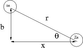
Notice

as [math]ze[/math] is scattered the horizontal component of the coulomb force ([math]F[/math]) flips direction; ie no horizontal force

[math]F_{vertical} = k \frac{zZe^2}{r^2} \sin(\theta) = k \frac{zZe^2}{r^2} \frac{b}{r}[/math]

where

k =[math]\frac{1}{4 \pi \epsilon_0}[/math]

r = distance between incident projectile and target atom

b= impact parameter of collision

Using the definition of Impulse one can determine the momentum change of [math]ze[/math] as

[math]\Delta p = \int F dt[/math]

Let's assume that the energy lost by the incident particle [math]ze[/math] is absorbed by an electron in the target atom. This energy may be cast in terms of the incident particles momentum change as

[math]\frac{(\Delta p)^2}{2m_e}[/math]

By calculating the change in momentum ([math]\Delta p[/math]) of the incident particle we can infer the amount of energy lost by the incident particle and absorbed one of the target materials atomic electrons.

[math]\Delta P = \int F dt = \int k \frac{zZe^2b}{r^3} dt[/math]

using [math]dt = \frac{dx}{v} = \frac{d x}{\beta c}[/math] we have

[math]= k \frac{zZe^2b}{\beta c} \int_{-\infty}^{+\infty} \frac{ dx}{(x^2+b^2)^{3/2}}[/math]

[math]=\frac{kzZe^2b}{\beta c b^2} \int_{-\infty}^{+\infty} \frac{ dx/b}{(1+\frac{x}{b^2})^{3/2}}[/math]

[math]\int_{-\infty}^{+\infty} \frac{ dx/b}{(1+\frac{x}{b^2})^{3/2}}=2[/math]

[math] \Delta p = \frac{2kzZe^2b}{\beta c b^2}[/math]

casting this in terms of the classical atomic electron radius [math]r_e[/math]

[math]r_e = \frac{k e^2}{m_e v^2} \sim \frac{k e^2}{m_e c^2}[/math] just equate [math]F = \frac{ke^2}{r_e^2} = m \frac{v^2}{r_e}[/math]

Then

[math] \Delta p = \frac{2zZr_e m_e c}{\beta b}[/math]

and

[math]\Delta E = \frac{(\Delta p)^2}{2m_e} = 2 \left ( \frac{r_e m_e}{\beta b}\right )^2 \frac {z^2 Z^2 c^2}{m_e}[/math] : [math]Z[/math] = 1 here because I shall assume the energy is lost to just the electron and the Atom is a spectator

Now let's calculate an expression representing the average energy lost for an incident particle traversing a material of some thickness.

Let

[math]P(\Delta E)[/math] = Probability of an interaction taking place which results in an energy loss [math]\Delta E[/math]

If we let

Z = Atomic Number = # electrons in target Atom = number of protons in an Atom

N = Avagadros number = [math]6.022 \times 10^{23} \frac{Atoms}{mol}[/math]

A = Atomic mass = [math]\frac{g}{mole}[/math]

[math]dP(\Delta E)[/math] = probability of hitting an atomic electron in the area of an annulus of radius ([math]b + db[/math]) with an energy transfer between [math]\Delta E[/math] and [math]\Delta E + d(\Delta E)[/math]

Then

[math]\frac{-dE }{dx}= \int_0^{\infty} dP(\Delta E) \Delta E[/math] = energy lost by the incident particle per distance traversed through the material

I am just adding up all the energy losses weighted by the probability of the energy loss to find the total energy loss.

[math]dP(\Delta E) = \frac{N}{A} d \sigma =\frac{N}{A} (2 \pi b db) Z[/math] : classically [math]\sigma = \pi b^2 ; d \sigma = 2\pi b db [/math]

[math]\Rightarrow \frac{-dE}{dx} = \int_0^{\infty} \frac{N}{A} (2 \pi b db) Z \Delta E = \frac{2 \pi N Z}{A} \int_0^{\infty} \Delta E b db[/math]

= [math]\frac{2 \pi N Z}{A} \int_0^{\infty} \left [ \frac{2 r_e^2 m_e c^2 z^2}{\beta^2 b^2}\right ] b db[/math]

= [math]4 \pi N r_e^2 m_e c^2 \frac{z^2 Z}{A \beta^2} \int_0^{\infty} \frac{db}{b}[/math]

=[math]\frac{\mathcal{K} }{A} \frac{z^2 Z}{\beta^2} \int_0^{\infty} \frac{db}{b}[/math]

where [math]\frac{\mathcal{K}}{A} = \frac{4 \pi N r_e^2 m_e c^2}{A} = 0.307 \frac{MeV cm^2}{g}[/math] if A=1

The limits of the above integral should be more physical in order to reflect the limits of the physics interaction. Let b_{min} and b_{max} represent the minimum and maximum possible impact parameter where the physics is discribed, as shown above, by the coulomb force.

What is [math]b_{min}[/math]?

if [math]b \rightarrow 0[/math] then [math]\frac{d E}{dx}[/math] diverges and the energy transfer [math]\rightarrow \infty : \Delta E \sim \frac{1}{b}[/math]. Physically there is a maximum energy that may be transferred before the physics of the problem changes (ie: nuclear excitation, jet production, ...). The de Borglie wavelength of the atom is used to estimate a value for [math]b_{min}[/math] such that

[math]b_{min} \sim \frac{1}{2} \lambda_{de Broglie} = \frac{h}{2p} = \frac{h}{2 \gamma m_e \beta c}[/math]

What is b_{max}?

As [math]b[/math] gets bigger the interaction is "softer" and longer. If the interaction time ([math]\tau_i[/math]) is so long that it is equivalent to an electron orbit ([math]\tau_R[/math]) then the atom looks more like it is neutrally charged. You move from an interaction in which the electron orbit is perturbed adiabatically such that there is no orbit change and the minimum amount of energy is transferred to no interaction taking place because the atom is neutral.

Let

[math]\tau_i = \frac{b_{max}}{v} (\sqrt{1-\beta^2})[/math] : fields at high velocities get Lorentz contracted

[math]\tau_R \equiv \frac{h}{I}[/math] : I [math]\equiv[/math] mean excitation energy of target material ( [math]E = h \nu = h/ \tau[/math])

Condition for [math]b_{max}[/math] :

[math]\tau_i = \tau_R[/math]

[math]\Rightarrow b_{max} = \frac{h \gamma \beta c}{I}[/math]

[math]-\frac{dE}{dx} = \frac{\mathcal{K} }{A} \frac{z^2 Z}{\beta^2} \int_0^{\infty} \frac{db}{b}[/math]

[math]= \frac{\mathcal{K} }{A} \frac{z^2 Z}{\beta^2} \ln \frac{b_{max}}{b_{min}}[/math]

[math]= \frac{\mathcal{K} }{A} \frac{z^2 Z}{\beta^2} \ln \frac{2 \gamma^2 m_e \beta^2 c^2}{I}[/math]

Example 5: Find [math]\frac{dE}{dx}[/math] for a 10 MeV proton hitting a liquid hydrogen ([math]LH_2[/math]) target

A = Z=z=1
[math]m_e c^2[/math] = 0.511 MeV
I = 21.6 eV : see solid data point From Figure 27.5 on pg 6 of PDG below.

Just need to know [math]\gamma[/math] and [math]\beta[/math]

"a 10 MeV proton" [math]\Rightarrow[/math] Kinetic Energy (K.E.) = 10 MeV = [math](\gamma - 1) mc^2[/math]

[math]\Rightarrow \gamma = \frac{K.E.}{mc^2} + 1 = \frac{10 MeV}{938 MeV} + 1 \sim 1 = \frac{1}{\sqrt{1-\beta^2}}[/math]

Proton is not relativistic

[math]v^2 = \frac{2 K.E.}{m} = \frac{2 \cdot 10 MeV}{938 MeV/c^2} = 2 \times 10^{-2} c^2 \Rightarrow \beta^2 = \frac{v^2}{c^2} = 2\times 10^{-2}[/math]

Plugging in the numbers:

[math]\frac{dE}{dx} = \left ( 0.307 \frac{MeV \cdot cm^2}{g}\right ) (1)^2 (1) \frac{1}{2 \times10^{-2}} \ln \left( \frac{2 (1) (0.511 MeV) (2 \times10^{-2})}{21.6 eV} \frac{10^6 eV}{MeV}\right)[/math]

[math]= 105 \frac{MeV cm^2}{g}[/math]

How much energy is lost after 0.3 cm?

[math]\rho_{LH_2}[/math] = 0.07 [math]\frac{g}{cm^3}[/math]

[math]\Delta E = (105 \frac{MeV cm^2}{g}) (0.07 \frac{g}{cm^3}) (0.3 cm)[/math] = 2.2 MeV

Bethe-Bloch Equation

While the classical equation above works in a limited kinematic regime, the Bethe-Bloch equation includes the corrections needed to cover most kinematic regimes for heavy particle energy loss.

[math]-\frac{dE}{dx} = \mathcal{K} z^2 \frac{Z}{A} \frac{1}{\beta^2} \left [ \frac{1}{2} \ln \left (\frac{2 m_2 c^2 \beta^2 \gamma^2 T_{max}}{I^2} \right) - \beta^2 - \frac{\delta}{2}\right ][/math]PDG reference Eq 27.1 pg 1

where

[math]T_{max} = \frac{2 m_e c^2 \beta^2 \gamma^2}{1+ \frac{2 \gamma m_e}{M} + \frac{m_e}{M}}[/math]

= Max K.E. transferable to the Target of mass [math]M[/math] in a single collision.

[math]-\beta^2[/math]

= correction for electron spin and very distant collisions which deform the electron atomic orbits each process reducing dE/dx by [math]\frac{\beta}{2}[/math]

[math]\frac{\delta}{2}[/math]

= density correction term: in the classical derivation the material is treated as just a system of [math]N[/math] atoms uniformly distributed in space. These Atoms, however, give the material polarizability which can reduce the electric field (dielectric).

GEANT 4 implementation

The GEANT4 file

source/processes/electromagnetic/standard/src/G4BetheBlockModel.cc

is used to calculate hadron energy loss.

line 132 [math]\Rightarrow[/math]

[math]-\frac{dE}{dx} = \log \left ( \frac{2 m_e c^2 \tau (\tau +2) E_{min}}{I^2}\right) - \beta^2 - (1 - \frac{E_{min}{E_{max}}[/math]