|
|
| (62 intermediate revisions by 2 users not shown) |
| Line 2: |
Line 2: |
| | | | |
| | =Sample Description= | | =Sample Description= |
| − | The sample was placed in an aluminum cylinder that was to be irradiated. The target components consisted of a nickel foil on the front of the cylinder with 2 pure selenium pellets under the foil, but still outside the cylinder. Inside the target there was burnt sagebrush ash, which was burned with a blowtorch, and selenium. Below are the masses of the components | + | The sample was placed in an aluminum cylinder that was to be irradiated. The target components consisted of a nickel foil on the front of the cylinder with 2 pure selenium pellets under the foil, but still outside the cylinder. Inside the target there was burnt sagebrush ash, which was place in an oven, and selenium. Below are the masses of the components |
| | | | |
| | Nickel Foil: 0.2783g | | Nickel Foil: 0.2783g |
| Line 18: |
Line 18: |
| | The Calibration for Detector A was done on the morning of 5/23/17 with the MPA software using the thorium rods (as the calibration was fairly close already) and the correction values were found to be Det A Intercept = -12.208800 slope =1.021270 | | The Calibration for Detector A was done on the morning of 5/23/17 with the MPA software using the thorium rods (as the calibration was fairly close already) and the correction values were found to be Det A Intercept = -12.208800 slope =1.021270 |
| | | | |
| − | | + | Se170063 Thin Window Analysis |
| | =Efficiency= | | =Efficiency= |
| | | | |
| Line 24: |
Line 24: |
| | | | |
| | =Nickel Information= | | =Nickel Information= |
| − | In finding the initial activity of the front nickel foil of this sample, look at the window from [1356,1368]. The method I used here was simply finding the number of counts within this window and subtracting the integral of the constant found by the fit. Below is a picture of the line of interest.
| |
| − |
| |
| − | [[File:170063 003 NickelSpectrum.png|200px]]
| |
| − |
| |
| − | Note that this spectrum is weighted by the inverse of the mass of the nickel. So the natural log of the activity is what we want to put in the .dat file to feed into root. Below is the math that I did to find these numbers
| |
| − |
| |
| − | <math> N = N_{total} - \int_{1356}^{1368} C dE </math>
| |
| − |
| |
| − |
| |
| − | After the number of counts have been found, I used the following formula for the error
| |
| − |
| |
| − | <math> \sigma_N = \sqrt{N} </math>
| |
| − |
| |
| − | So now we have the number of counts for the line of interest and its associated error, so we must convert this into an activity, correct for the efficiency, and take the natural log.
| |
| − |
| |
| − | <math> A_t = \frac{N_t}{t} </math>
| |
| − |
| |
| − | <math> \sigma_{A_t} = \frac{\sigma_{N}}{t} </math>
| |
| | | | |
| − | <math> A'_t = \frac{A_t}{\epsilon} </math>
| + | [[Se170063 Nickel Investigation]] |
| − | | |
| − | <math> \sigma_{A'_t} = \frac{\sigma_{A_t}}{\epsilon} </math>
| |
| − | | |
| − | Now we can simply take the natural log of the efficiency corrected activity. To find the error after taking the natural log, use
| |
| − | | |
| − | <math> \sigma_{\ln{A'_t}} = \frac{\sigma_{A'_t}}{A'_t} </math>
| |
| − | | |
| − | | |
| − | Below is the plot for the activity and half life of the nickel foil
| |
| − | | |
| − | [[File:170063 003 HalfLifePlot.png|200px]] | |
| − | | |
| − | | |
| − | Using the slope of this graph, we can find that the half life is
| |
| − | | |
| − | <math> t_{\frac{1}{2}} = \frac{\ln{2}}{\lambda} = 35.71 hours </math>
| |
| − | | |
| − | <math> \sigma_{t_{\frac{1}{2}}} = \frac{\ln{2}*\sigma_{lambda}}{\lamdba^2} </math>
| |
| | | | |
| | =Activity and Half Life= | | =Activity and Half Life= |
| − | The window used during this investigation was [110,118]. I used the script on daq1 /data/IAC/Se/May2017/5_25_17/Eff.C which fits lines of interest to a Gaussian function plus a constant. Once this function is found, the constant is integrated across the window of interested, then subtracted out of the original equation. After that the Gaussian is integrated across the window which gives the total number of counts for the peak of interest (in this case it is the 93 keV line of Se-81). To find the error in the counts, I increased the value for the standard deviation by a factor of 3 and integrated that function across the region of interest and subtracted that value from the original number of counts. Below is an example of a spectrum seen when using Eff.C
| + | [[Se170063 Activity And Half Life]] |
| | | | |
| − | [[File:170063 SeSoilMix Spectrum.png|200px]] | + | The method that has given the most acceptable results is given in [[Se170063 Thin Window Analysis]] |
| | | | |
| − | Note that the amplitude of the Gaussian fit is slightly higher than the actual maximum number of counts. To fix this, I simply used ROOT to find the maximum in the given window with
| |
| | | | |
| − | Int_t max=0;
| + | Compare Rates between Two pure SE samples Irradiated at same time and measured using same detector with samples at the same location |
| − | hist1->GetXaxis()->SetRange(RangeMin,RangeMax);
| |
| − | max = hist1 -> GetMaximum();
| |
| − | cout << "Maximum is " << max << endl;
| |
| | | | |
| − | After that I forced the amplitude term in the Gaussian to be that maximum via
| + | [[Se_5-25-17-RateCompare_OuterSe]] |
| | | | |
| − | p0Gauss -> SetParameter(0,max);
| + | =Alternative Method= |
| | | | |
| − | Once the raw number of counts and the error has been obtained, before entering the value into a .dat file a few modifications were made to that number. The first and simplest modification is to convert the number of counts into activity simply by dividing by the time duration of the measurement. In other words
| + | [[Se170063 Activity and HL Alternate]] |
| | | | |
| − | <math>A(t) = \frac{N(t)}{t} </math>
| + | =Corrected Alternative method= |
| | + | The files used for this analysis are in the directory /data/IAC/Se/May2017/5_25_17/Se_Activity_SysOffset_Mix |
| | | | |
| − | Since the radioactive decay equation is given by
| + | To begin, I have corrected the mixture to have a factor of 0.62, which is the mystery factor throwing of all of these analyses. The histogram is also weighted by the mass. The weight added to the histogram is |
| | | | |
| − | <math>A(t) = A_0e^{-\lambda*t}</math> | + | <math> h1 -> Fill(evt.Chan,\frac{1}{0.0523*0.62}) </math> |
| | | | |
| − | So to get a linear equation, simply take the natural log of both sides, which gives | + | So the true number of counts has indeed been weighted here. Now I want to try to test every different method that was suggested. So first I am going to weight the mixture by the mystery factor of 0.62, and leave my Gaussian fits as wide as they were previously. The gaussians will probably be made more compact if the mystery factor does not alleviate the problem. The first step is to find the number of counts within the window of interest. Below is the process I used to determine the number of counts and the error associated with it. First begin by plotting the histogram using the ROOT program Eff.C, which is shown below. |
| | | | |
| − | (1) <math>\ln{(A(t))} = \ln{(A_0)} - \lambda*t </math>
| + | [[File:170063 Spec Weighted.png|200px]] |
| | | | |
| − | So we take the natural log of the activity and input that value into the .dat file. To propagate the error we take the error in the number of counts and divide by the time to put the error in units of Hertz. After that, since we are taking the natural log, we must use the standard error propagation formula, which is given by
| + | Now take the integral given in the stats box and subtract the background to get the number of counts. Here the number of counts would be |
| | | | |
| − | (2) <math>\sigma_{\ln{A}} = \sqrt{(\frac{\partial \ln{A}}{\partial A})^2 * \sigma_A^2 } = \frac{1}{A}*\sigma_A = \frac{t}{N}*\frac{\sigma_N}{t} = \frac{\sigma_N}{N} </math>
| + | <math> 927800 - 47670 = 880130 Counts </math> |
| | | | |
| | + | Now I can convert this error into an activity by dividing by the time, which is 300 seconds in this case. After that take the natural log of the quotient. |
| | | | |
| − | Once the activity and its associated error have been computed, put the values into a .dat file with 3 columns. The first column is the time elapsed for the measurement, the second column is the natural log of the activity, and finally the third column is the associated error found as outlined above.
| + | <math> \ln{\frac{880130}{300}} = 7.984042428 </math> |
| | | | |
| | + | Now to find the error we can notice that the standard deviation here is 0.6238. The procedure is to expand the window by one or two standard deviations and find the difference in the number of counts in the original window. Due to the binning here I have decided to expand the window by 1 channel on each side, which is roughly 2 standard deviations. A picture is given below. |
| | | | |
| − | Once the .dat file has been created, simply change the script /data/IAC/Se/May2017/5_25_17/LB_WeightedFit.C to read in the new .dat file and run the script on ROOT. Doing so will give a plot such as the one below
| + | [[File:170063 Spec ExpandedWindow.png|200px]] |
| | | | |
| − | [[File:170063 PureSe HalfLife Plot.png|200px]]
| + | Now we do a similar method to find the number of counts within this window. |
| | | | |
| | + | <math> 1017000 - 46810 = 970190 Counts </math> |
| | | | |
| − | This plot gives parameters of the linear equation (1). The next step in the process is to find the half life of the sample. To do so recall that
| + | Now take the difference between the original window's number of counts and the expanded window's number of counts. |
| | | | |
| − | <math> t_{\frac{1}{2}} = \frac{\ln{2}}{\lambda} = \frac{\ln{2}}{0.000207} = 3,348.54 Seconds \rightarrow 55.8090 Minutes </math> | + | <math> 970190 - 880130 = 90060 Counts </math> |
| | | | |
| | + | Now to propagate this error we must divide this number by the original number of counts. |
| | | | |
| − | Now we must propagate the error in the half life. Even though the error in the decay constant says that it is zero in the plot, by looking at the root output, it can be seen that the error is actually
| + | <math> \frac{90060}{880130} = 0.1023257928 </math> |
| − | | |
| − | <math> 5.91816*10^{-9} s^{-1} </math> (See if this can be fixed)
| |
| − | | |
| − | To propagate the error, use the standard propagation of error formula
| |
| − | | |
| − | <math> \sigma_{t_{\frac{1}{2}}} = \sqrt{(\frac{\partial t_{\frac{1}{2}}}{\partial \lambda})^2 * \sigma_\lambda ^2} = \frac{\ln{2}}{\lambda^2}*\sigma_\lambda = 0.095446 s \rightarrow 0.001591 Minutes</math>
| |
| − | | |
| − | which gives us a half life of
| |
| − | | |
| − | <math> t_{\frac{1}{2}} = 55.8090 \pm 0.0016 </math> Minutes
| |
| − | | |
| − | The accepted value of the half life of Se-81 is
| |
| − | | |
| − | <math> 57.28 \pm 0.02 Minutes </math>
| |
| − | | |
| − | Note that these two values do not overlap. This means that there could be some systematic error within the measurement systems.
| |
| − | | |
| − | Now, to find the activity of the sample when it was measured, we use the other parameter given by ROOT. Note that the value given is
| |
| − | | |
| − | <math> \ln{A_{measure}} </math>
| |
| − | | |
| − | This means we must exponentiate to get the initial activity parameter to continue
| |
| − | | |
| − | <math> e^{\ln{A_{measure}}} = e^{5.34637} = 209.845 Hz </math>
| |
| − | | |
| − | The associated error to the activity at the time of measurement can be found as well. Since we are exponentiating and the exponential function is its own derivative, the error can be written as
| |
| − | | |
| − | <math> \sigma_{A_t} = e^{\ln{A_t}}*\sigma_{\ln{A_t}} = 0.003 Hz </math>
| |
| − | | |
| − | | |
| − | which means that the activity of the Pure Selenium sample at the beginning of the measurement was
| |
| − | | |
| − | <math>A_t = 209.845 \pm 0.003 Hz </math>
| |
| − | | |
| − | Now note that the pure sample was measured second in the split run file. This means that the activity at the beginning of the measurement must be backtracked to when the mixture of ash and selenium was measured, which was 400 seconds prior. To do this, solve the radioactive decay equation for the initial activity.
| |
| − | | |
| − | <math> A_0 = A_t*e^{\lambda*t} = (209.845)*e^{0.00207*400} = 227.960 Hz </math>
| |
| − | | |
| − | | |
| − | Now to propagate the error using the standard error propagation formula using 0.5 seconds for the uncertainty in the time.
| |
| − | | |
| − | <math> \sigma_{A_0} = \sqrt{(\frac{\partial A_0}{\partial A_t})^2\sigma_{A_t}^2 + (\frac{\partial A_0}{\lambda})^2\sigma_{\lambda}^2 + (\frac{\partial A_0}{\partial t})^2\sigma_{t}} = \sqrt{e^{2\lambda t}\sigma_{A_t}^2 + A_{t}^2t^2e^{2\lambda t}\sigma_{\lambda}^2 + A_t^2\lambda^2e^{2\lambda t}\sigma_t^2} = \sqrt{1.06209\times 10^{-5} + 2.91212 \times 10^{-7} + 5.56669 \times 10^{-4} } = 0.024 </math>
| |
| − | | |
| − | Which means that the activity of the Pure selenium sample, corrected to be the activity at the same time that the mixture was measure is
| |
| − | | |
| − | <math>A_0 = 227.960 \pm 0.024 Hz </math>
| |
| − | | |
| − | | |
| − | Now moving on to the Se-Torch Ash mixture, we can apply a similar analysis to find the initial activity.
| |
| − | | |
| − | Below is the plot for the half life of the mixture
| |
| − | | |
| − | [[File:170063 Mix HalfLifePlot.png|200px]]
| |
| − | | |
| − | Now to find the half life use
| |
| − | | |
| − | <math> t_{\frac{1}{2}} = \frac{\ln{2}}{\lambda} = \frac{\ln{2}}{0.000181} = 3829.54 Seconds \rightarrow 63.8257 Minutes </math>
| |
| − | | |
| − | Propagating the error in the half life gives
| |
| − | | |
| − | <math> \sigma_{t_{\frac{1}{2}}} = \sqrt{(\frac{\partial t_{\frac{1}{2}}}{\partial \lambda})^2 * \sigma_\lambda ^2} = \frac{\ln{2}}{\lambda^2}*\sigma_\lambda = 0.2397 s \rightarrow 0.004 Minutes</math>
| |
| − | | |
| − | Even though the error in the decay constant cannot be seen on the plot, it is given in to ROOT window to be
| |
| − | | |
| − | <math>\sigma_{\lambda} = 1.13316 \times 10^{-8} </math>
| |
| − | | |
| − | | |
| − | which mmeans that the half life of the mixed sample is
| |
| − | | |
| − | <math> t_{\frac{1}{2}} = 63.8257 \pm 0.004 Minutes </math>
| |
| − | | |
| − | Now moving on to the activity of the sample. Doing a similar analysis as above we can find the activity of the sample at the beginning of the measurement
| |
| − | | |
| − | <math> e^{\ln{A_{t}}} = e^{4.016235} = 55.4919 Hz </math>
| |
| − | | |
| − | and the error is given by
| |
| − | | |
| − | <math> \sigma_{A_t} = e^{\ln{A_t}}*\sigma_{\ln{A_t}} = 0.0014 Hz </math>
| |
| − | | |
| − | So the activity at the beginning of the measurement is
| |
| − | | |
| − | <math> 55.4918 \pm 0.0014 Hz </math>
| |
| − | | |
| − | Now taking the ratio of the activities we get
| |
| − | | |
| − | <math> \frac{N_{Mix}}{N_{Pure}} = \frac{55.4919}{227.960} = 0.24 </math>
| |
| − | | |
| − | =Alternative Method=
| |
| − | | |
| − | While analyzing the data it became clear that the amplitude of the gaussian fit did not match the amplitude of the peak of interest. Below is an example
| |
| | | | |
| − | [[File:170063 PureSeSpectrum HighAmplitude.png|200px]]
| + | This method was repeated for the next set of runs that make the data file. The numbers are in a table below. |
| | | | |
| − | This can be corrected in multiple ways. The first way is to use the draw panel to manually adjust the amplitude of the gaussian. The second way (which is the way I used) is to find the maximum value of a histogram in a range of interest using ROOT.
| + | {| border="3" cellpadding="5" cellspacing="0" |
| | + | || || 0 <t< 300 sec || 730 < t < 1020 sec || 1480 < t < 1775 || 2250 < t < 2550 sec || 3050 < t < 3300 sec || 3775 < t < 4050 sec || 4480 < t < 4770 sec |
| | + | |- |
| | + | ||Original Window Counts || 880200 || 716200 ||617100 || 545800 ||394100 || 362000 || 346300 |
| | + | |- |
| | + | || Original Window Background (Integrated) || 381379 || 267608 || 215260 || 189665 || 143921 || 137541 || 128197 |
| | + | |- |
| | + | ||Original Window Difference || 498821 || 448592 || 401850 || 356135|| 250179 || 224459 || 218103 |
| | + | |- |
| | + | ||Expanded Window Counts || 970900 || 782600 || 671300 || 593100 || 426700 ||395400 ||378100 |
| | + | |- |
| | + | ||Expanded Window Background || 468138 || 333633 || 269025 || 236476 || 173353 ||170089 || 159644 |
| | + | |- |
| | + | ||Expanded Window Difference || 502762 || 448967 || 402275 || 356624 ||253347 || 225311 || 218456 |
| | + | |- |
| | + | ||Error in counts || 3941 || 375 || 425 || 489 || 3168 || 852 || 353 || |
| | + | |- |
| | + | ||.dat file entry || 7.416220118 +/- 0.0079006297 || 7.343988145 +/- 0.0008359489264 || 7.216858801 +/- 0.0010576086 || 7.079282677 +/- 0.0013730748 || 6.908471023 +/- 0.012662933 || 6.704677244 +/- 0.0037957934 || 6.622841784 +/- 0.0016185014 |
| | + | |- |
| | + | |} |
| | | | |
| − | Int_t max=0;
| + | Below is the graph that contains the information about the initial activity and the half life |
| − | hist1->GetXaxis()->SetRange(RangeMin,RangeMax);
| |
| − | max = hist1 -> GetMaximum();
| |
| | | | |
| − | p0Gauss -> SetParameter(0,max);
| + | [[File:170063 WindowExpand WideGauss HLPlot.png|200px]] |
| | | | |
| − | This will force the amplitude to be the maximum of the histogram in the region of interest. In previous attempts I simply fit a gaussian function plus a constant so the gaussian would be shifted up to the background. In this attempt, I subtracted the background constant value from the amplitude to find a new background corrected amplitude. Using this amplitude, the mean and standard deviation parameters given by ROOT, I used Mathematica to do the following integral
| + | The slope of the line is -0.00019198 +/- 4.13511e^-7, which gives a half life of |
| | | | |
| − | <math> \int_{110}^{118}{(A_{corrected})*e^{\frac{-(x-\bar{x})^2}{2*\sigma^2}}dx} </math> | + | <math> t_{\frac{1}{2}} = \frac{\ln{2}}{\lambda}\rightarrow 60.18 minutes </math> |
| | | | |
| − | This integral would give me the number of counts. For the error I used the square root of the counts since this is indeed a counting experiment. The linear fits are shown below.
| + | While the error is |
| | | | |
| − | [[File:170063 Mix HalfLife Plot.png|200px]]
| + | <math> \sigma_{t_{\frac{1}{2}}} = \frac{\ln{2}*\sigma_{\lambda}}{\lambda^2} \rightarrow 0.13 minutes </math> |
| − | [[File:170063 PureSe HalfLife Corrected.png|200px]]
| |
| | | | |
| | + | The constant value given by the plot is 7.4918 +/- 0.000927611, which gives an initial activity of |
| | | | |
| − | Using the method of calculation outlined above, the half life was found to be
| + | <math> A_0 = e^{7.4918} = 1793.28 Hz </math> |
| | | | |
| − | <math> 62.79 \pm 0.99 Minutes </math> for the mix
| + | and an error of |
| | | | |
| − | <math> 54.31 \pm 0.41 Minutes </math> for the pure selenium sample | + | <math> e^{7.4918}*\sigma_{A} = 1.66 Hz </math> |
| | | | |
| − | The activities were found to be
| + | Now correcting for the efficiency we have |
| | | | |
| − | <math> 172.99 \pm 2.33 Hz </math> for the Pure Se Sample | + | <math> A_0^' = \frac{A_0}{\epsilon} = \frac{1793.28}{0.007} = 256182.8571 Hz </math> |
| | | | |
| − | <math> 40.39 \pm 0.27 Hz </math> for the mixture
| + | While the error is |
| | | | |
| − | This gives a ratio of 0.23.
| + | <math> \sigma_{A_0^'} = \frac{A_0}{\epsilon^2}*\sigma_{\epsilon} = 402.57 Hz </math> |
| | | | |
| − | This is the third method that I have tried and gotten very close results. Using the incorrect higher amplitude method I got a ratio of 0.25. Using the corrected amplitude method with the gaussian plus constant fit I got 0.24. Now using the new corrected amplitude along with Mathematica I got 0.23. This seems to tell me that the ratio is indeed around 0.25, even though it is supposed to be 0.5. Looking at just a simple spectrum (which will be the first measurement taken for each sample, the number of counts is significantly higher.
| + | Below are the related pages for this sample using this method of window expansion: |
| | | | |
| − | [[File:170063 MixSpec CountDiffExample.png|200px]] | + | [[Se170063 Nickel Foil Wide Gauss Window Expansion]] |
| − | [[File:170063 PureSeSpec CountDiffExample.png|200px]]
| |
| | | | |
| − | Now note that the Mixture was measured first for 5 minutes, the norm-background gives 7517.2 for the corrected amplitude while the Pure Se sample gives 24304.7 for the corrected amplitude. So roughly 6 minutes later, the pure selenium sample's peak counts is about 3 times higher than that of the mixture.
| + | [[Se170063 Pure Se Wide Gauss Window Expansion]] |
| | | | |
| | =Runlist= | | =Runlist= |
PAA_Selenium/Soil_Experiments#Selenium_Sample_Analysis
Sample Description
The sample was placed in an aluminum cylinder that was to be irradiated. The target components consisted of a nickel foil on the front of the cylinder with 2 pure selenium pellets under the foil, but still outside the cylinder. Inside the target there was burnt sagebrush ash, which was place in an oven, and selenium. Below are the masses of the components
Nickel Foil: 0.2783g
Outer Se Pellets: 0.0971g
Sage Ash: 0.5111g
Inner Se Pellets: 0.0523g
Energy
LB May Calibration 2017
The Calibration for Detector A was done on the morning of 5/23/17 with the MPA software using the thorium rods (as the calibration was fairly close already) and the correction values were found to be Det A Intercept = -12.208800 slope =1.021270
Se170063 Thin Window Analysis
Efficiency
LB May 2017 Det A Efficiency
Nickel Information
Se170063 Nickel Investigation
Activity and Half Life
Se170063 Activity And Half Life
The method that has given the most acceptable results is given in Se170063 Thin Window Analysis
Compare Rates between Two pure SE samples Irradiated at same time and measured using same detector with samples at the same location
Se_5-25-17-RateCompare_OuterSe
Alternative Method
Se170063 Activity and HL Alternate
Corrected Alternative method
The files used for this analysis are in the directory /data/IAC/Se/May2017/5_25_17/Se_Activity_SysOffset_Mix
To begin, I have corrected the mixture to have a factor of 0.62, which is the mystery factor throwing of all of these analyses. The histogram is also weighted by the mass. The weight added to the histogram is
[math] h1 -\gt Fill(evt.Chan,\frac{1}{0.0523*0.62}) [/math]
So the true number of counts has indeed been weighted here. Now I want to try to test every different method that was suggested. So first I am going to weight the mixture by the mystery factor of 0.62, and leave my Gaussian fits as wide as they were previously. The gaussians will probably be made more compact if the mystery factor does not alleviate the problem. The first step is to find the number of counts within the window of interest. Below is the process I used to determine the number of counts and the error associated with it. First begin by plotting the histogram using the ROOT program Eff.C, which is shown below.
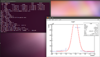
Now take the integral given in the stats box and subtract the background to get the number of counts. Here the number of counts would be
[math] 927800 - 47670 = 880130 Counts [/math]
Now I can convert this error into an activity by dividing by the time, which is 300 seconds in this case. After that take the natural log of the quotient.
[math] \ln{\frac{880130}{300}} = 7.984042428 [/math]
Now to find the error we can notice that the standard deviation here is 0.6238. The procedure is to expand the window by one or two standard deviations and find the difference in the number of counts in the original window. Due to the binning here I have decided to expand the window by 1 channel on each side, which is roughly 2 standard deviations. A picture is given below.
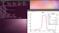
Now we do a similar method to find the number of counts within this window.
[math] 1017000 - 46810 = 970190 Counts [/math]
Now take the difference between the original window's number of counts and the expanded window's number of counts.
[math] 970190 - 880130 = 90060 Counts [/math]
Now to propagate this error we must divide this number by the original number of counts.
[math] \frac{90060}{880130} = 0.1023257928 [/math]
This method was repeated for the next set of runs that make the data file. The numbers are in a table below.
|
0 <t< 300 sec |
730 < t < 1020 sec |
1480 < t < 1775 |
2250 < t < 2550 sec |
3050 < t < 3300 sec |
3775 < t < 4050 sec |
4480 < t < 4770 sec
|
| Original Window Counts |
880200 |
716200 |
617100 |
545800 |
394100 |
362000 |
346300
|
| Original Window Background (Integrated) |
381379 |
267608 |
215260 |
189665 |
143921 |
137541 |
128197
|
| Original Window Difference |
498821 |
448592 |
401850 |
356135 |
250179 |
224459 |
218103
|
| Expanded Window Counts |
970900 |
782600 |
671300 |
593100 |
426700 |
395400 |
378100
|
| Expanded Window Background |
468138 |
333633 |
269025 |
236476 |
173353 |
170089 |
159644
|
| Expanded Window Difference |
502762 |
448967 |
402275 |
356624 |
253347 |
225311 |
218456
|
| Error in counts |
3941 |
375 |
425 |
489 |
3168 |
852 |
353 |
|
| .dat file entry |
7.416220118 +/- 0.0079006297 |
7.343988145 +/- 0.0008359489264 |
7.216858801 +/- 0.0010576086 |
7.079282677 +/- 0.0013730748 |
6.908471023 +/- 0.012662933 |
6.704677244 +/- 0.0037957934 |
6.622841784 +/- 0.0016185014
|
Below is the graph that contains the information about the initial activity and the half life
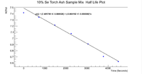
The slope of the line is -0.00019198 +/- 4.13511e^-7, which gives a half life of
[math] t_{\frac{1}{2}} = \frac{\ln{2}}{\lambda}\rightarrow 60.18 minutes [/math]
While the error is
[math] \sigma_{t_{\frac{1}{2}}} = \frac{\ln{2}*\sigma_{\lambda}}{\lambda^2} \rightarrow 0.13 minutes [/math]
The constant value given by the plot is 7.4918 +/- 0.000927611, which gives an initial activity of
[math] A_0 = e^{7.4918} = 1793.28 Hz [/math]
and an error of
[math] e^{7.4918}*\sigma_{A} = 1.66 Hz [/math]
Now correcting for the efficiency we have
[math] A_0^' = \frac{A_0}{\epsilon} = \frac{1793.28}{0.007} = 256182.8571 Hz [/math]
While the error is
[math] \sigma_{A_0^'} = \frac{A_0}{\epsilon^2}*\sigma_{\epsilon} = 402.57 Hz [/math]
Below are the related pages for this sample using this method of window expansion:
Se170063 Nickel Foil Wide Gauss Window Expansion
Se170063 Pure Se Wide Gauss Window Expansion
Runlist
Table with dates and filename and locations on daq1
LB_May_2017_Irradiation_Day#10.25_Se_Soil_Mix
PAA_Selenium/Soil_Experiments#Selenium_Sample_Analysis


