Sadiq Proposal Defense

Emittance

What is Emittance

In accelerator physics, Cartesian coordinate system was used to describe motion of the accelerated particles. Usually the z-axis of Cartesian coordinate system is set to be along the electron beam line as longitudinal beam direction. X-axis is set to be horizontal and perpendicular to the longitudinal direction, as one of the transverse beam direction. Y-axis is set to be vertical and perpendicular to the longitudinal direction, as another transverse beam direction.

For the convenience of representation, we use [math]z[/math] to represent our transverse coordinates, while discussing emittance. And we would like to express longitudinal beam direction with [math]s[/math]. Our transverse beam profile changes along the beam line, it makes [math]z[/math] is function of [math]s[/math], [math]z~(s)[/math]. The angle of a accelerated charge regarding the designed orbit can be defined as:

[math]z'=\frac{dz}{ds}[/math]

If we plot [math]z[/math] vs. [math]z'[/math], we will get an ellipse. The area of the ellipse is an invariant, which is called Courant-Snyder invariant. The transverse emittance [math]\epsilon[/math] of the beam is defined to be the area of the ellipse, which contains 90% of the particles <ref name="MConte08"> M. Conte and W. W. MacKay, “An Introduction To The Physics Of Particle Accelera tors”, World Scientifc, Singapore, 2008, 2nd Edition, pp. 257-330. </ref>.

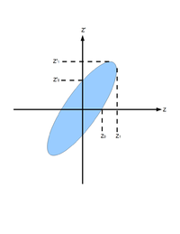
Fig.1 Phase space ellipse <ref name="MConte08"></ref>.

Measurement of Emittance with Quad Scanning Method

In quadrupole scan method, a quadrupole and a Yttrium Aluminum Garnet (YAG ) screen was used to measure emittance. Magnetic field strength of the quadrupole was changed in the process and corresponding beam shapes were observed on the screen. Transfer matrix of a quadrupole magnet under thin lens approximation:

[math] \left( \begin{matrix} 1 & 0 \\ -k_{1}L & 1 \end{matrix} \right)=\left( \begin{matrix} 1 & 0 \\ -\frac{1}{f} & 1 \end{matrix} \right) [/math]

Here, [math]k_{1} L[/math] is quadrupole strength, [math]L[/math] is quadrupole magnet thickness, and f is quadrupole focal length. [math] k_{1} L \gt 0 [/math] for x-plane, and [math] k_{1} L \lt 0 [/math] for y-plane. Transfer matrix of a drift space between quadrupole and screen:

[math] \mathbf{S} = \left( \begin{matrix} S_{11} & S_{12} \\S_{21} & S_{22} \end{matrix} \right)=\left( \begin{matrix} 1 & l \\ 0 & 1 \end{matrix} \right) [/math]

Here, [math]l[/math] ([math]S_{12}[/math]) is the distance from the center of the quadrupole to the screen. Transfer matrix of the scanned region is:

[math] \mathbf{M} = \mathbf{SQ} = \begin{pmatrix} m_{11} & m_{12} \\ m_{21} & m_{22} \end{pmatrix}= \begin{pmatrix} S_{11} & S_{12} \\ S_{21} & S_{22} \end{pmatrix} \begin{pmatrix} 1 & 0 \\ -k_1L & 1 \end{pmatrix}= \begin{pmatrix} S_{11} - k_1LS_{12} & S_{12} \\ S_{21} - k_1L S_{22} & S_{22} \end{pmatrix} [/math]

[math]\mathbf{M}[/math] is related with the beam matrix [math]\mathbf{\sigma}[/math] as:

[math] \mathbf{ \sigma_{screen}} = \mathbf{M \sigma_{quad} M^T} = \begin{pmatrix} m_{11} & m_{12} \\ m_{21} & m_{22} \end{pmatrix} \begin{pmatrix} \sigma_{quad, 11} & \sigma_{quad, 12} \\ \sigma_{quad, 21} & \sigma_{quad, 22} \end{pmatrix} \begin{pmatrix} m_{11} & m_{12} \\ m_{21} & m_{22} \end{pmatrix} [/math]

Since:

[math] \sigma_{x}=\sqrt{\epsilon_x\beta},~\sigma_{x'}=\sqrt{\epsilon_x\gamma},~\sigma_{xx'}={-\epsilon_x\alpha} [/math]

[math] \mathbf{ \sigma} = \begin{pmatrix} \sigma_{11} & \sigma_{12} \\ \sigma_{21} & \sigma_{22} \end{pmatrix} = \begin{pmatrix} \sigma_{x}^2 & \sigma_{xx'} \\ \sigma_{xx'} & \sigma_{x'}^2 \end{pmatrix} [/math]

So, [math]\mathbf{\sigma}[/math] matrix can be written as: [math] \mathbf{\sigma}_{quad} = \begin{pmatrix} \sigma_{quad, x} & \sigma_{quad, xx'} \\ \sigma_{quad, xx'} & \sigma_{quad, x,} \end{pmatrix} = \epsilon_{rms, x} \begin{pmatrix} \beta & -\alpha \\ -\alpha & \gamma \end{pmatrix} [/math]

Substituting this give:

[math] \mathbf{ \sigma_{screen}} = \mathbf{M \sigma_{quad} M^T} = \begin{pmatrix} m_{11} & m_{12} \\ m_{21} & m_{22} \end{pmatrix} \epsilon_{rms, x} \begin{pmatrix} \beta & -\alpha \\ -\alpha & \gamma \end{pmatrix} \begin{pmatrix} m_{11} & m_{12} \\ m_{21} & m_{22} \end{pmatrix} [/math]

Dropping off subscript "rms" on emittance [math]\epsilon_{rms, x}[/math]: [math] \sigma_{screen, 11}=\sigma_{screen, x}^2=\epsilon_x (m_{11}^2\beta - 2m_{12}m_{11}\alpha+m_{12}^2\gamma) [/math]

Using [math]\mathbf{\sigma}[/math] matrix relations:

[math] \sigma_{x}={\epsilon_x\beta},~\sigma_{12}={-\epsilon_x\alpha},~{\epsilon_x\gamma}=\epsilon_x \frac{1+\alpha^2}{\beta}=\frac{\epsilon_x^2+\sigma_{12}^2}{\sigma_{11}} [/math]

Here [math]\sigma_{x}[/math] is [math]\sigma_{screen, x}[/math]. We got:

[math] \sigma_{x}^2=m_{11}^2 \sigma_{11} + 2m_{12}m_{11} \sigma_{12} + m_{12}^2 \frac{\epsilon_x^2+\sigma_{12}^2}{\sigma_{11}} [/math]

[math] \sigma_{x}^2=\sigma_{11} \left(m_{11}^2 + 2m_{11}m_{12}\frac{\sigma_{12}}{\sigma_{11} }+ m_{12}^2\frac{\sigma_{12}^2}{\sigma_{11}^2}\right) + m_{12}\frac{\epsilon_x^2}{\sigma_{11}} [/math]

[math] \sigma_{x}^2=\sigma_{11}\left(m_{11} + m_{12}\frac{\sigma_{12}}{\sigma_{11} }\right)^2 + m_{12}\frac{\epsilon_x^2}{\sigma_{11}} [/math]

Recall:

[math] m_{11} = S_{11}-kLS_{12}~~~~~~m_{12}=S_{12} [/math]

Substituting and reorganizing result in:

[math] \sigma_{x}^2=\sigma_{11} {S_{12}^2}\left(kL - \left( \frac{S_{11}}{S_{12}} + \frac{\sigma_{12}}{\sigma_{11}} \right) \right)^2 + S_{12}^2\frac{\epsilon_x^2}{\sigma_{11}} \lt math\gt Introducing constants \lt math\gt A[/math],[math]B[/math], and [math]C[/math]

[math] A = \sigma_{11} {S_{12}^2},~~B = \frac{S_{11}}{S_{12}} + \frac{\sigma_{12}}{\sigma_{11}},~~C = S_{12}^2\frac{\epsilon_x^2}{\sigma_{11}} [/math]

This will simplify equation to:

[math] \sigma_{x}^2=A(kL - B)^2 + C = A(kL)^2 - 2AB(kL)+(C+AB^2) [/math]

It is easy to see that:

[math] \epsilon = \frac{\sqrt{AC}}{S_{12}^2} [/math]

By changing quadrupole magnetic field strength $k$, we can change beam sizes [math]\sigma_{x,y}[/math] on the screen. We make projection to the x, y axes, then fit them with Gaussian fittings to extract rms beam sizes, then plot vs [math]\sigma_{x,y}[/math] vs [math]k_{1}L[/math]. By Fitting a parabola we can find constants [math]A[/math],[math]B[/math], and [math]C[/math], and get emittances.

References

<references/>

Using APA reference style.

File:Emittance.tex

Go back: Positrons