Quantum Mechanics Review
- Debroglie - wave particle duality
| Particle |
Wave
|
| [math]E[/math] |
[math]\hbar \omega = h \nu[/math]
|
| [math]P[/math] |
[math]\hbar k = \frac{h}{\lambda}[/math]
|
- Heisenberg uncertainty relationship
- [math]\Delta x \Delta p_x \ge \frac{\hbar}{2}[/math]
- [math]\Delta E \Delta t \ge \frac{\hbar}{2}[/math]
- [math]\Delta \ell_z \Delta \phi \ge \frac{\hbar}{2}[/math] where [math]\phi[/math] characterizes the location of [math]\ell[/math] in the x-y plane
- Classical: [math]\frac{p^2}{2m} + V(r) = E[/math]
- Quantum (Schrodinger Equation): [math]-\frac{\hbar^2}{2m}\nabla^2 \Psi + V(r) \Psi = i\hbar \frac{\partial \Psi}{\partial t}[/math]
- [math]\;\;\;\;\;\; p_x \rightarrow -i \hbar \frac{\partial}{\partial x} \;\;\; E \rightarrow i \hbar \frac{\partial}{\partial t}[/math]
- E = energy eigenvalues
- [math]\Psi(x,t) = \psi(x)e^{-\omega t}[/math] = eigenvectors [math]\omega=\frac{E}{\hbar}[/math]
- [math]P = \int_{x_1}^{x_2}\Psi^*(x,t) \Psi(x,t)[/math] = probability of finding the particle (wave packet) between [math]x_1[/math] and [math]x_2[/math]
- [math]\Psi^*[/math] = complex conjugate [math](i \rightarrow -i)[/math]
- [math]\lt f\gt = \int \Psi^* f \Psi dx =\lt \Psi^*| f| \Psi\gt [/math] = average (expectation) value of observable [math]f[/math] after many measurements of [math]f[/math]
- example: [math]\lt p_x\gt =\int \Psi^* \left ( -i\hbar \frac{\partial}{\partial x}\right ) \Psi dx[/math]
- Constraints on Quantum solutions
- [math]\psi[/math] is continuous accross a boundary : [math]\lim_{\epsilon \rightarrow 0} \left [ \psi(a+\epsilon) - \psi(a-\epsilon)\right ] =0[/math] and [math]\lim_{\epsilon \rightarrow 0} \left [ \left(\frac{\partial \psi}{\partial x} \right )_{a+\epsilon} - \left(\frac{\partial \psi}{\partial x} \right )_{a-\epsilon}\right ] =0[/math] ( if [math]V(x)[/math] is infinite this second condition can be violated)
- the solution is normalized:[math]\int \psi^* \psi dx =\lt \psi^* | \psi \gt =1[/math]
- Current conservation: the particle current density associated with the wave function [math]\Psi[/math] is given by
- [math]j = \frac{\hbar}{2mi} \left ( \Psi^* \frac{\partial \Psi}{\partial x}-\Psi \frac{\partial \Psi^*}{\partial x}\right )[/math]
Schrodinger Equation
1-D problems
Free particle
If there is no potential field (V(x) =0) then the particle/wave packet is free. The wave function is calculated using the time-dependent Schrodinger equation:
- [math]-\frac{\hbar^2}{2m} \nabla^2 \Psi(x,t) + 0 = i\hbar\frac{\partial \Psi(x,t)}{\partial t}[/math]
Using separation of variables Let:
- [math]\Psi(x,t) = \psi(x) f(t)[/math]
Substituting we have
- [math]-\frac{\hbar^2}{2m} f(t) \frac{d^2 \psi(x)}{d x^2} = i \hbar \psi(x) \frac{d f(t)}{d t}[/math]
reorganizing you can move all functions of [math]x[/math] on one side and [math]t[/math] on the other suggesting that both sides equal some constant which we will call [math]E[/math]
- [math]-\frac{\hbar^2}{2m} \frac{1}{\psi(x)} \frac{d^2 \psi(x)}{d x^2} = i \hbar \frac{1}{f(t)} \frac{d f(t)}{d t} \equiv E[/math]
Solving the temporal (t) part:
- [math]\frac{1}{f(t)} \frac{d f(t)}{d t} = -\frac{i E}{\hbar} \Rightarrow f(t) = e^{-iEt/\hbar}[/math] : just integrate this first order diff eq.
Solving the spatial (x) part:
- [math]\frac{1}{\psi(x)} \frac{d^2 \psi(x)}{d x^2} =- \frac{2m E}{\hbar^2}[/math]
Such second order differential equations have general solutions of
- [math]\psi(x) = A e^{ikx} + B e^{-ikx}[/math] where [math]k^2 = \frac{2mE}{\hbar^2}[/math]
Now put everything together
- [math]\Psi(x,t) = \psi(x) f(t) = \left (A e^{ikx} + B e^{-ikx} \right ) e^{-iEt/\hbar}[/math]
- [math]= A e^{i(kx-\omega t)} + B e^{-i(kx-\omega t)}[/math]
- Notice
- [math]\lt \Psi(x,t) | \Psi(x,t)\gt = \lt \psi(x)| \psi(x)\gt \Rightarrow [/math]the wave function amplitude does not change with time
- also, if the operator for an observable A does not change in time, then
- [math]\lt \Psi(x,t) | A | \Psi(x,t)\gt = \lt \psi(x)| A| \psi(x)\gt \Rightarrow [/math] even though particles are not stationary they are in a quantum state which does not change with time (unlike decays).
- the term of amplitude[math] A[/math] represents a wave traveling in the +x direction while the second term represents a wave traveling in the -x direction.
- Example
- consider a free particle traveling in the +x direction
- Then
- [math]\Psi(x,t) = A e^{i(kx-\omega t)} : kx-\omega t =0 \Rightarrow x= \omega t/k = vt \Rightarrow[/math] wave moving to right
- if the particles are coming from a source at a rate of[math] j[/math] particles/sec then
- [math]j = \frac{\hbar}{2mi} \left ( \Psi^* \frac{\partial \Psi}{\partial x}-\Psi \frac{\partial \Psi^*}{\partial x}\right )[/math]
- [math]= \frac{\hbar}{2mi} \left ( A^*A[ik] - A A^* [-ik]\right ) = \frac{\hbar k}{m} \left ( A^*A\right )= \frac{\hbar k}{m} \left | A \right |^2[/math]
- [math]\Rightarrow A = \sqrt{\frac{mj}{\hbar k}}[/math]
Step Potential
Consider a 1-D quantum problem with the Step potential V(x) defined below where [math]V_o \gt 0[/math]
- [math]V(x) =\left \{ {0 \;\;\;\; x \lt 0 \atop V_o \;\;\;\; x\gt 0} \right .[/math]
Break these types of problems into regions according to how the potential is defined. In this case there will be 2 regions
x<0
When x<0 then V =0 and we have a free particle system which has the solution given above.
- [math]\Psi_1(x,t) = \psi_1(x) f(t) = \left (A e^{ikx} + B e^{-ikx} \right ) e^{-iEt/\hbar}[/math]
- [math]= A e^{i(kx-\omega t)} + B e^{-i(kx-\omega t)}[/math] where [math]k^2 =\frac{2mE}{\hbar^2}[/math] and [math]\omega =\frac{E}{\hbar}[/math]
x>0
- [math]-\frac{\hbar^2}{2m} \nabla^2 \Psi_2(x,t) + V_o = i\hbar\frac{\partial \Psi_2(x,t)}{\partial t}[/math]
- [math]-\frac{\hbar^2}{2m} \frac{\partial^2 \Psi_2(x,t)}{\partial x^2} + V_o = i\hbar\frac{\partial \Psi_2(x,t)}{\partial t}[/math]
separation of variables: [math]\Psi_2(x,t) = \psi_2(x)f(t)[/math]
- [math]-\frac{\hbar^2}{2m} f(t)\frac{\partial^2 \psi_2(x)}{\partial x^2} + V_o\psi(x)f(t) = i\hbar \psi_2(x)\frac{\partial f(t)}{\partial t}[/math]
- [math]-\frac{\hbar^2}{2m} \frac{1}{\psi_2(x)}\frac{\partial^2 \psi_2(x)}{\partial x^2} + V_o = i\hbar \frac{1}{f(t)}\frac{\partial f(t)}{\partial t} \equiv E =[/math] Constant
The time dependent part of the problem is the same as the free particle solution. Only the spatial part changes because the Potential is not time dependent.
- [math]-\frac{\hbar^2}{2m} \frac{1}{\psi_2(x)}\frac{\partial^2 \psi_2(x)}{\partial x^2} =E - V_o = [/math] Constant
- [math] \frac{\partial^2 \psi_2(x)}{\partial x^2} =-\frac{2m}{\hbar^2}(E - V_o) \psi_2(x) [/math]
If [math]E \gt V_o[/math] then we have a wave that traverses the step potential partly reflected and partly transmitted, otherwise it will be reflected back and the part that is transmitted will tunnel through the barrier attenuated exponentially for x>0.
Here is how it works out mathematically
[math]E \gt V_o[/math]
For the case where [math]E \gt V_o[/math]:
- [math] \frac{\partial^2 \psi_2(x)}{\partial x^2} =-\frac{2m}{\hbar^2}(E - V_o) \psi_2(x) \equiv -k_2^2 \psi_2(x)\lt 0 [/math]
- [math] \frac{\partial^2 \psi_2(x)}{\partial x^2} \equiv -k_2^2 \psi_2(x)\lt 0 \Rightarrow[/math]SHM solutions
The above Diff. Eq. is the same form as the free particle but with a different constant
- Let
- [math]\psi_2(x) = Ce^{ik_2x} + De^{-ik_2x}[/math]
Now apply Boundary conditions:
- [math]\psi(x=0) = \psi_2(x=0)[/math]
- [math]A + B = C + D : e^{\pm i 0} = 1[/math]
and
- [math]\frac{\partial \psi}{\partial x}|_{x=0} = \frac{\partial \psi_2}{\partial x}|_{x=0}[/math]
- [math]k(A-B) = k_2 (C-D)[/math]
We now have a system of 2 equations and 4 unknowns which we can't solve.
- Notice
- The coefficient "D" in the above system represent the component of [math]\psi_2[/math] represent a wave moving from the right towards x=0. If we assume the free particle encountered this step potential by originating from the left side, then there is no way we can have a component of [math]\psi_2[/math] moving to the left. Therefore we set [math]D=0[/math].
- The coefficient A represent the incident plane wave on the barrier. The remaining coefficients B and C represent the reflected and transmitted components of the traveling wave, respectively.
- Know our system of equations is
- [math]A+B =C[/math]
- [math]A -B = \frac{k_2}{k} C[/math]
- If I assume that the coefficient A is known (I know what the amplitude of the incoming wave is) then I can solve the above system such that
- [math]A+B = C = (A-B)\frac{k}{k_2}[/math]
- [math]B=A\frac{1-\frac{k_2}{k}}{1+\frac{k_2}{k}}[/math]
similarly
- [math]C = A+B = A\left (1+ \frac{1-\frac{k_2}{k}}{1+\frac{k_2}{k}} \right ) = \frac{2A}{1+\frac{k_2}{k}}[/math]
Reflection (R) and Transmission (T) Coefficients
- [math]R\equiv \frac{j_{reflected}}{j_{incident}} = \frac{|B|^2}{|A|^2} = \left ( \frac{1-\frac{k_2}{k}}{1+\frac{k_2}{k}} \right )^2[/math]
- [math]T\equiv \frac{j_{transmitted}}{j_{incident}} = \frac{C^*ik_2C + Cik_2C^*}{A^*ikA + AikA^*} = \frac{k_2 |C|^2}{k |A|^2} =\frac{4 \frac{k_2}{k}}{\left ( 1 + \frac{k_2}{k} \right )^2} [/math]
- [math]=1 - R =1-\left ( \frac{1-\frac{k_2}{k}}{1+\frac{k_2}{k}} \right )^2 =\frac{ \left( 1+\frac{k_2}{k} \right )^2 - \left ( 1-\frac{k_2}{k}\right )^2}{\left ( 1+\frac{k_2}{k}\right )^2}=\frac{4 \frac{k_2}{k}}{\left ( 1 + \frac{k_2}{k} \right )^2} [/math]
[math]E \lt V_o[/math]
- [math] \frac{\partial^2 \psi_2(x)}{\partial x^2} =-\frac{2m}{\hbar^2}(E - V_o) \psi_2(x) \gt 0[/math]
- Let
- [math]k_3 \equiv \sqrt{\frac{2m}{\hbar^2}(V_o-E)}[/math]
Then
- [math] \frac{\partial^2 \psi_3(x)}{\partial x^2} =k_3 \psi_3(x) \gt 0 \Rightarrow[/math] exponential decay
- Assume solution
- [math]\psi_3 = G e^{k_3x} + Fe^{-k_3x}[/math]
- Recall the solution for x<0
- [math]\psi_1(x,t) = A e^{ikx} + B e^{-ikx}[/math] where [math]k^2 =\frac{2mE}{\hbar^2}[/math]
- Apply Boundary conditions
If [math]x \rightarrow \infty[/math]
Then [math]e^{\infty} \rightarrow \infty \Rightarrow G =0[/math]
- [math]\psi_3 = Fe^{-k_3x}[/math]
- Continuous conditions at x=0
- [math]A+B = F[/math]
- [math]ik(A-B) = -k_3F[/math]
Assuming A is known we have 2 equations and 2 unknowns again
- [math]A+B = \frac{ik}{-k_3} (A-B)[/math]
- [math]B=-A\left(\frac{1+\frac{ik}{k_3}}{1-\frac{ik}{k_3}} \right) = A\left(\frac{1-\frac{ik_3}{k}}{1+\frac{ik_3}{k}} \right)[/math]
- [math]F = A\left (1-\left(\frac{1-\frac{ik_3}{k}}{1+\frac{ik_3}{k}}\right) \right)=\frac{2A}{1+\frac{ik_3}{k}}[/math]
Reflection (R) and Transmission (T) Coefficients=
- [math]R\equiv \frac{j_{reflected}}{j_{incident}} = \frac{|B|^2}{|A|^2} = \left(\frac{1-\frac{ik_3}{k}}{1+\frac{ik_3}{k}} \right)\left(\frac{1-\frac{ik_3}{k}}{1+\frac{ik_3}{k}} \right)^*[/math]
- [math]=\left(\frac{1-\frac{ik_3}{k}}{1+\frac{ik_3}{k}} \right)\left(\frac{1-\frac{-ik_3}{k}}{1+\frac{-ik_3}{k}} \right) = 1[/math]
- [math]T\equiv \frac{j_{transmitted}}{j_{incident}} = \frac{F^*k_3F - Fk_3F^*}{A^*ikA + AikA^*} =0 =1-R [/math]
- Evanescent waves
- Waves like [math]\psi_3[/math] which carry no current. There is a finite probability of penetrating the barrier (tunneling) but no net current is transmitted. A feature which separates Quantum mechanics from classical.
Rectangular Barrier Potential
Barrier potentials are 1-D step potentials of height [math](V_o \gt 0)[/math] which have a finite step width:
- [math]V(x) =0 \;\;\; x\lt 0[/math]
- [math]V(x) =\left \{ {V_o \;\;\;\; 0 \le x \le a \atop 0 \;\;\;\; x\gt a} \right .[/math]
We now have 3 regions in space to solve the schrodinger equation
We know from the free particle solutions that on the left and right side of the barrier we should have
- [math]\psi_1 = = A e^{ikx} + B e^{-ikx} \;\;\; x \lt 0[/math]
- [math]\psi_3 = = F e^{ikx} + G e^{-ikx} \;\;\; x \gt a[/math]
where
- [math]k^2= \frac{2mE}{\hbar^2}[/math]
But in the region [math]0 \le x \le a[/math] we have the save type of problem as the step in which the solution depends on the Energy of the system with respect to the potential. One solution for the [math]E\gt V_o[/math] (oscilatory) system and one for the [math]E\lt V_o[/math] (exponetial decay) system.
- [math]\psi_2 = \left \{ {= Ce^{ik_2x} + De^{-ik_2x} \;\;\;\; E\gt V_o \atop = Ce^{k_3x} + De^{-k_3x} \;\;\;\; E \lt V_o } \right .[/math]
where
- [math]k_2^2=\frac{2m(E-V_o)}{\hbar^2}\;\;\; k_3^2=\frac{2m(V_o-E)}{\hbar^2}[/math]
[math]E \gt V_o[/math]
For the case where [math]E \gt V_o[/math]:
Before we set [math]D =0[/math] because there wasn't a wave moving to the left towards the [math]x=0[/math] interface. The rectangular barrier though could have a wave reflect back form the [math]x=a[/math] interface.
- Apply Boundary conditions
- [math]\psi_1(x=0) = \psi_2(x=0)[/math]
- [math]A + B = C + D : [/math]
and
- [math]\psi_2(x=a) = \psi_3(x=a)[/math]
- [math]Ce^{ik_2a} + De^{-ik_2a} = Fe^{ika} + Ge^{-ika} [/math]
and
- [math]\frac{\partial \psi_1}{\partial x}|_{x=0} = \frac{\partial \psi_2}{\partial x}|_{x=0}[/math]
- [math]k(A-B) = k_2 (C-D)[/math]
and
- [math]\frac{\partial \psi_2}{\partial x}|_{x=a} = \frac{\partial \psi_3}{\partial x}|_{x=a}[/math]
- [math]k_2(Ce^{ik_2a}-De^{-ik_2a}) = k (Fe^{ika}-Ge^{-ika})[/math]
We now have a system of 4 equations
and 6 unknowns (A,B,C, D, F and G).
But:
- [math]G=0[/math] : no source for wave moving to left when x>a
If we treat [math]A[/math] as being known (you know the incident wave amplitude) then we have 4 unknowns (B,C,D, and F) and the 4 equations:
- [math]A + B = C + D : [/math]
- [math]k(A-B) = k_2 (C-D)[/math]
- [math]Ce^{ik_2a} + De^{-ik_2a} = Fe^{ika} : [/math]
- [math]k_2(Ce^{ik_2a}-De^{-ik_2a}) = k Fe^{ika}[/math]
Transmission
- [math]T \equiv \frac{|F|^2}{|A|^2}[/math] = the transmission coefficient
To find the ration of F to A
- solve the last 2 equations for C & D in terms of F
- solve the first 2 equations for A in terms C and D
- 3.)substitute your values for C and D from the last 2 equations so you have the ratio of B/A in terms of F/A
- 1.)solve the last 2 equations
- [math]Ce^{ik_2a} + De^{-ik_2a} = Fe^{ika} : [/math]
- [math]Ce^{ik_2a}-De^{-ik_2a} = \frac{k}{k_2} Fe^{ika}[/math]
for C and D
- [math]2Ce^{ik_2a} =Fe^{ika}\left ( 1+\frac{k}{k_2} \right)[/math]
- [math]2De^{-ik_2a} =Fe^{ika}\left ( 1-\frac{k}{k_2} \right)[/math]
- 2.) solve the first 2 equations for B in terms of C & D
- [math]A + B = C + D : [/math]
- [math]A-B = \frac{k_2}{k} (C-D)[/math]
for A in terms of C and D
- [math]2B=C \left ( 1- \frac{k_2}{k}\right ) + D\left ( 1+ \frac{k_2}{k}\right )[/math]
- [math]=\frac{F}{2}e^{i(k-k_2)a}\left ( 1+\frac{k}{k_2}\right ) \left ( 1- \frac{k_2}{k}\right ) +\frac{F}{2}e^{i(k+k_2)a}\left ( 1-\frac{k}{k_2} \right)\left ( 1+ \frac{k_2}{k}\right )[/math]
- [math]=\frac{F}{2}e^{i(k-k_2)a}\left ( \frac{k}{k_2}-\frac{k_2}{k}\right ) +\frac{F}{2}e^{i(k+k_2)a}\left ( - \frac{k}{k_2}+\frac{k_2}{k}\right )[/math]
- [math]\Rightarrow \frac{B}{A} = \frac{Fe^{ika}}{4A}\left[ \left ( e^{-ik_2a} -e^{ik_2a}\right ) \frac{k}{k_2} +\left ( -e^{-ik_2a} -e^{ik_2a}\right ) \frac{k_2}{k} \right ][/math]
- [math]= -\frac{Fe^{ika}}{4A} \left [ 2i\sin(k_2a) \frac{k}{k_2} -2 i\sin(k_2a)\frac{k_2}{k}\right ][/math]
- 3.) Find Reflection Coeff in terms of Transmission Coeff
- [math]\frac{B}{A}=- \frac{F}{A}\frac{ie^{ika}\sin(k_2a)}{2} \left [ \frac{k^2-k_2^2}{kk_2} \right ][/math]
- [math]T +R = \frac{|F|^2}{|A|^2} + \frac{|B|^2}{|A|^2} = \frac{|F|^2}{|A|^2} + \frac{F^*}{A^*}\frac{-ie^{-ika}\sin(k_2a)}{2} \left [ \frac{k^2-k_2^2}{kk_2} \right ]\frac{F}{A}\frac{ie^{ika}\sin(k_2a)}{2} \left [ \frac{k^2-k_2^2}{kk_2} \right ] = 1[/math]
- [math]\Rightarrow \frac{|F|^2}{|A|^2} \left (1 + \frac{\sin^2(k_2a)}{4}\left [ \frac{k^2-k_2^2}{kk_2} \right ]^2 \right) = 1[/math]
or
- [math]T = \frac{|F|^2}{|A|^2} = \frac{1}{\left (1 + \frac{\sin^2(k_2a)}{4}\left [ \frac{k^2-k_2^2}{kk_2} \right ]^2 \right) }[/math]
since
- [math]k^2= \frac{2mE}{\hbar^2} \;\;k_2^2= \frac{2m(E-V_o)}{\hbar^2}[/math]
Then
- [math]T = \frac{|F|^2}{|A|^2} = \frac{1}{\left (1 + \frac{\sin^2(k_2a)}{4}\left [ \frac{V_o^2}{E(E-V_o)} \right ] \right) }[/math]
3-D problems
Infinite Spherical Well
What is the solution to Schrodinger's equation for a potential V which only depends on the radial distance (r) from the origin of a coordinate system?
- [math]V =\left \{ {0 \;\;\;\; r\lt a \atop \infty \;\;\;\; r\gt a} \right .[/math]
Such a potential lends itself to the use of a Spherical coordinate system in which the schrodinger equation has the form
- [math]\hat{H}\psi(r,\theta,\phi) = E\psi(r,\theta,\phi)[/math]
- [math]-\frac{\hbar^2}{2m}\nabla^2 \psi(r,\theta,\phi)+V\psi(r,\theta,\phi) = E\psi(r,\theta,\phi)[/math]
In spherical coordinates
- [math]\nabla^2 = \frac{1}{r} \frac{\partial^2}{\partial r^2} r + \frac{1}{r^2} \left ( \frac{1}{\sin(\theta)} \frac{\partial}{\partial \theta} \sin(\theta)\frac{\partial}{\partial \theta} + \frac{1}{\sin^2(\theta)}\frac{\partial^2}{\partial \phi^2}\right )[/math]
- Note
- [math]\frac{1}{r} \frac{\partial^2}{\partial r^2} r = \frac{1}{r} \frac{\partial}{\partial r} r \left ( \frac{1}{r} \frac{\partial}{\partial r} \right ) = \left (\frac{1}{r} \frac{\partial}{\partial r} \right)^2 \equiv -\left ( \frac{\hat{p}_r}{\hbar} \right )^2[/math]
- [math]\left ( \frac{1}{\sin(\theta)} \frac{\partial}{\partial \theta} \sin(\theta)\frac{\partial}{\partial \theta} + \frac{1}{\sin^2(\theta)}\frac{\partial^2}{\partial \phi^2}\right ) \equiv -\frac{\hat{L}^2}{\hbar^2}[/math]
so
- [math]\hat{H}\psi(r,\theta,\phi) = \left ( \frac{\hat{p}_r^2}{2m} + \frac{\hat{L}^2}{2mr^2} + V \right ) \psi(r,\theta,\phi)= E\psi(r,\theta,\phi)[/math]
Using separation of variables:
- [math]\psi(r,\theta,\phi) \equiv R(r) \Theta(\theta) \Phi(\phi)[/math]
which we can also write as
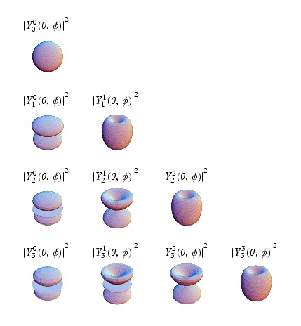
- [math]\psi(r,\theta,\phi) \equiv R(r) Y_{l,m}(\theta, \phi)[/math]
where
- [math]Y_{l,m}(\theta, \phi) \equiv \Theta(\theta) \Phi(\phi)[/math]
Substitute
- [math]\frac{1}{2mR(r)} \hat{p}_r^2 R(r)+ \frac{1}{2mr^2Y_{l,m}} \hat{L}^2 Y_{l,m}= E-V[/math]
V=0
We have a constant on the right hand side so the left hand side must also be constant
- [math]\frac{1}{2mr^2Y_{l,m}} \hat{L}^2 Y_{l,m} = \frac{l(l+1)\hbar^2}{2mr^2} =[/math]a "centrifugal" barrier which keeps particles away from r=0
substituting
- [math]\frac{1}{2mR(r)} \hat{p}_r ^2R(r) + \frac{l(l+1)\hbar^2}{2mr^2} = E-V[/math]
In the region where V=0
- [math]\frac{1}{\hbar^2R(r)}\hat{p}_r^2 R(r) + \frac{l(l+1)}{r^2} = \frac{2m}{\hbar^2}E[/math]
The Radial equation becomes
- [math]\left ( \frac{\hat{p}_r^2}{\hbar^2}+ \frac{l(l+1)}{r^2} \right ) R(r)= \left ( \frac{-1}{r} \frac{\partial^2}{\partial r^2} r + \frac{l(l+1)}{r^2} \right ) R(r)=\frac{2mE}{\hbar^2}R(r)[/math]
Let
- [math]k^2 = \frac{2mE}{\hbar^2}[/math]
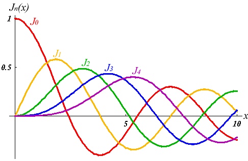
Then we have the "spherical Bessel"differential equation with the solutions:
- [math]j_l(kr) = \left (\frac{-r}{k} \right ) ^l \left (\frac{1}{r} \frac{d}{dr} \right )^l j_o (kr)[/math]
where
- [math]j_o(kr) = \frac{sin(kr)}{kr}[/math]
[math]Y_{l,m}[/math] and [math] j_l[/math] Table
| [math]l[/math] |
[math] m_l [/math] |
[math] j_l[/math] |
[math]Y_{l,m_l}[/math]
|
| 0 |
0 |
[math]\frac{\sin(kr)}{kr} = \frac{1}{2ikr} \left ( e^{ikr}-e^{-ikr} \right)[/math] |
[math]\sqrt{\frac{1}{4 \pi}}[/math]
|
| 1 |
0 |
[math]\frac{\sin(kr)}{(kr)^2} -\frac{\cos(kr)}{kr}[/math] |
[math]\sqrt{\frac{3}{4 \pi}}\cos(\theta)[/math]
|
|
[math]\pm[/math] 1 |
|
[math]\mp \sqrt{\frac{3}{8 \pi}}\sin(\theta)e^{\pm i \phi}[/math]
|
| 2 |
0 |
[math]\left ( \frac{3}{(kr)^3} - \frac{1}{kr} \right )\sin(kr) -\frac{3\cos(kr)}{(kr)^2}[/math] |
[math]\sqrt{\frac{5}{16 \pi}}(3\cos^2(\theta)-1)[/math]
|
|
[math]\pm[/math] 1 |
|
[math]\mp \sqrt{\frac{15}{8 \pi}}\sin(\theta)\cos(\theta)e^{\pm i \phi}[/math]
|
|
[math]\pm[/math] 2 |
|
[math]\mp \sqrt{\frac{15}{32 \pi}}\sin^2(\theta)e^{\pm 2 i \phi}[/math]
|
The general solution for the 3-D spherical infinite potential well problem is
- [math]\psi_{k,l,m}(r,\theta,\phi) = j_l(kr) Y_{l,m}(\theta, \phi)[/math] = eigen function(s)
where
- [math]k,l,m[/math] are quantization number and [math]E_k = \frac{\hbar^2 k^2}{2m} =[/math] quantum energy level = eigen state(s)
Energy Levels
To find the Energy eignevalues we need to know the value for "k". We apply the boundary condition
- [math]j_l(kr)= 0 [/math] at [math]r=a[/math]
to determine the "nodes" of [math]j_l[/math]; ie value of [math]ka[/math] so if you tell me the size of the well then I can tell you the value of k which will satisfy the boundary conditions. This means that "k" is not a "real" quantum number in the sense that it takes on integral values.
We simple label states with an integer [math](n)[/math] representing the [math]n^{th}[/math] zero crossing via:
- [math]| n,l\gt = j_l(ka) Y_{l,m_l}[/math]
For example:
- In the [math] l =0[/math] case
- [math]j_o(ka) =\frac{sin(ka)}{ka} = 0 [/math]when [math](ka) = \pi, 2\pi, 3\pi, 4\pi, ...[/math]
- You arbitrarily label these state as [math]n=1 \Rightarrow (ka) =\pi \;\;\;\; k = \pi/a \;\;\;\;\; E_0=\frac{\hbar^2 (\pi)^2}{2ma^2}, n=2 \Rightarrow (ka) = 2\pi [/math]
- [math]|1,0\gt = j_o(\pi r/a) Y_{0,0} \;\;\; E=E_0[/math]
- [math]|2,0\gt = j_o(2\pi r/a) Y_{0,0};\;\; E=2^2E_0 = 4E_0[/math]
- [math]|3,0\gt = j_o(3\pi r/a) Y_{0,0};\;\; E=3^2E_0=9E_0[/math]
- [math]|4,0\gt = j_o(4\pi r/a) Y_{0,0};\;\; E=4^2E_0=16E_0[/math]
- In the [math] l =1[/math] case
- [math]|1,1\gt = j_1(4.49 r/a) Y_{1,m_l}\;\;\; E=\left(\frac{4.49}{\pi}\right )^2E_0=2.04E_0[/math]
- [math]|2,1\gt = j_1(7.73 r/a) Y_{1,m_l}\;\;\; E=\left(\frac{7.73}{\pi}\right )^2E_0=6.05E_0[/math]
- [math]|3,1\gt = j_1(10.9 r/a) Y_{1,m_l}\;\;\; E=\left(\frac{10.9}{\pi}\right )^2E_0=12.04E_0[/math]
- [math]|4,1\gt = j_1(14.07 r/a) Y_{1,m_l}\;\;\; E=\left(\frac{14.07}{\pi}\right )^2E_0=20.1E_0[/math]
- Notice
- The angular momentum is degenerate for each level making the degeneracy for each energy [math]= 2l+1[/math]
File:EnergyLevel3-DInfinitePotentialWell.jpg
Simple Harmonic Oscillator
The potential for a Simple Harmonic Oscillator (SHM) is:
- [math]V(r) = \frac{1}{2} kr^2[/math]
This potential is does not depend on any angles. It's a central potential. Our solutions for Y_{l,m} from the 3-D infinite well potential will work for the SHM potential as well! All we need to do is solve the radial differential equation:
- [math]\frac{1}{R(r)}\hat{p}_r^2 R(r) + \frac{l(l+1)}{r^2} = \frac{2m}{\hbar^2}\left ( E - \frac{1}{2} kr^2 \right )[/math]
- [math]\left ( \frac{-1}{r} \frac{\partial^2}{\partial r^2} r + \frac{l(l+1)}{r^2} \right ) R(r)= \frac{2m}{\hbar^2}\left ( E - \frac{1}{2} kr^2 \right )R(r)[/math]
or
- [math]\frac{\partial^2}{\partial r^2} R(r) +\frac{2}{r} \frac{\partial}{\partial r} R(r) + \left ( \frac{2m}{\hbar^2}\left ( E - \frac{1}{2} kr^2 \right) -\frac{l(l+1)}{r^2}\right ) R(r)= 0[/math]
When solving the 1-D harmonic oscillator solutions were found which are of the form
- [math]\psi_x(x) = A_n e^{-x^2/2} H_n(x)[/math]
where
- [math]H_n(x) = (-1)^ne^{x^2} \frac{d^n}{dx^n} e^{-x^2}[/math]
If you construct the solution
- [math]\psi(x,y,z) = \psi(x) \psi(y) \psi(z) \sim e^{x^2/2+y^2/2+z^2/2} f(x,y,z) \sim e^{r^2/2} f(x,y,z)[/math]
Assume R(r) may be written as
- [math]R(r) = G(r) e^{-r^2/2}[/math]
substituting this into the differential equation gives
- [math]\frac{\partial^2 G}{\partial r^2} + \left ( \frac{2}{r} - \alpha r\right ) \frac{\partial G}{\partial r} + \left ( \lambda - \beta - \frac{l(l+1)}{r^2}\right ) G(r)= 0[/math]
The above differential equation can be solved using a power series solution
- [math]G = \sum_i^\infty a_ir^i[/math]
After performing the power series solution; ie find a recurrance relation for the coefficents a_i after substituting into the differential equation and require the coefficent of each power of r to vanish.
You arrive at a soultion of the form
- [math]\psi(r,\theta,\phi) \equiv R(r) Y_{l,m}(\theta, \phi) = e^{-r^2/2} G_{l,n} Y_{l,m}(\theta, \phi) [/math]
where
- [math]\ G_{l,n} =[/math] polynomial in [math]r[/math] of degree [math]n[/math] in which the lowest term in [math]r[/math] is [math]r^l[/math]
these polynomials are solutions to the differential equation
- [math]r^2\frac{\partial^2 G}{\partial r^2} + 2\left ( r-r^3\right ) \frac{\partial G}{\partial r} + \left ( 2nr^2- l(l+1)\right ) G(r)= 0[/math]
if you do the variable substitution
- [math]t = r^2[/math]
you get
- [math]t\frac{\partial^2 S}{\partial t^2} + \left ( l + \frac{3}{2} -t \right ) \frac{\partial S}{\partial t} + k S= 0[/math]
the above differential equation is called the "associated" Laguerre differential equation with the Laguerre polynomials as its solutions.
The following table gives you the Radial wave functions for a few SHO states:
| [math]n[/math] |
[math] l[/math] |
[math]E_n (\hbar \omega_o )[/math] |
[math]R(r)[/math]
|
| 0 |
0 |
[math]\frac{3}{2} [/math] |
[math]= \frac{2 \alpha^{3/2}}{\pi^{1/4}} e^{- \alpha^2 r^2/2}[/math]
|
| 1 |
1 |
[math]\frac{5}{2} [/math] |
[math]= \frac{2\sqrt{2} \alpha^{3/2}}{\sqrt{3} \pi^{1/4}} \alpha r e^{- \alpha^2 r^2/2}[/math]
|
| 2 |
0 |
[math]\frac{7}{2} [/math] |
[math]= \frac{2\sqrt{2} \alpha^{3/2}}{\sqrt{3} \pi^{1/4}} (\frac{3}{2} -\alpha^2 r^2 e^{- \alpha^2 r^2/2}[/math]
|
| 2 |
2 |
|
[math]= \frac{4 \alpha^{3/2}}{\sqrt{15} \pi^{1/4}} \alpha^2 r^2 e^{- \alpha^2 r^2/2}[/math]
|
| 3 |
1 |
[math]\frac{9}{2} [/math] |
[math]= \frac{4 \alpha^{3/2}}{\sqrt{15} \pi^{1/4}} (\frac{5}{2} \alpha r -\alpha^3 r^3 e^{- \alpha^2 r^2/2}[/math]
|
- Note
- Again there is a degeneracy of [math]2l+1[/math] for each [math]l[/math]
- Again E is independent of [math]l[/math] (central or constant potentials)
- if [math]n[/math] is odd [math]l[/math] is odd and if [math]n[/math] is even[math] l[/math] is even
- multiple values of [math]l[/math] occur for a give [math]n[/math] such that [math]l \le n[/math]
- The degeneracy is [math]\frac{1}{2} (n+1) (n+2)[/math] because of the above points
The Coulomb Potential for the Hydrogen like atom
The Coulomb potential is defined as :
- [math]V(r) = -\frac{Ze^2}{4 \pi \epsilon_0 r} [/math]
where
- [math]Z =[/math] atomic number
- [math]e =[/math] charge of an electron
- [math]\epsilon_0=[/math] permittivity of free space = [math]8.85 \times 10^{-12} Coul^2/(N m^2)[/math]
This potential does not depend on any angles. It's a central potential. Our solutions for [math]Y_{l,m}[/math] from the 3-D infinite well potential will work for the Coulomb potential as well! All we need to do is solve the radial differential equation:
- [math]\frac{1}{R(r)}\hat{p}_r^2 R(r) + \frac{l(l+1)}{r^2} = \frac{2m}{\hbar^2}\left ( E + \frac{k}{r} \right )[/math]
- [math]\left ( \frac{-1}{r} \frac{\partial^2}{\partial r^2} r + \frac{l(l+1)}{r^2} \right ) R(r)= \frac{2m}{\hbar^2}\left ( E + \frac{k}{r} \right )R(r)[/math]
or
- [math]\frac{1}{r}\frac{\partial^2}{\partial r^2} rR(r) + \left ( \frac{2m}{\hbar^2}\left ( E + \frac{k}{r} \right) -\frac{l(l+1)}{r^2}\right ) R(r)= 0[/math]
Radial Equation
Use the change of variable to alter the differential equiation
Let
- [math]G(r) \equiv r R(r)[/math]
Then the differential equation becomes:
- [math]\frac{\partial^2}{\partial r^2} G(r) + \left ( \frac{2m}{\hbar^2}\left ( E + \frac{k}{r} \right) -\frac{l(l+1)}{r^2}\right ) G(r)= 0[/math]
Consider the case where [math]|V| \gt |E| \Rightarrow[/math] (Bound states)
Bound state also imply that the eigen energies are negative
- [math]E = - |E|[/math]
Let
- [math]\kappa^2 \equiv \frac{2m |E|}{\hbar^2}[/math]
- [math]\rho \equiv 2 \kappa r[/math]
- [math]\lambda \equiv \left ( \frac{Ze^2 m }{\kappa \hbar^2} \right ) = Z \sqrt{\frac{\mathcal{R}}{|E|}}[/math]
- [math]\mathcal{R} = \frac{me^4}{2\hbar^2} = \frac{\hbar^2}{2m a_o^2} =1.09737316 \times 10^7\frac{1}{m} =[/math] Rydberg's constant
- [math]a_o = \frac{\hbar^2}{me^2} = 5.291772108 \times 10^{-11} m= 52918 fm =[/math] Bohr Radius
- [math]\frac{\partial^2}{\partial \rho^2} G(r) - \frac{l(l+1)}{\rho^2}G(r) + \left ( \frac{\lambda}{\rho} -\frac{1}{4} \right) G(r)= 0[/math]
Boundary conditions
- if [math]\rho[/math] is large then the diff equation looks like
- [math]\frac{\partial^2}{\partial \rho^2} G(r) -\frac{1}{4} G(r)= 0[/math]
- [math]\Rightarrow G(r) \sim Ae^{-\rho/2} + B e^{\rho/2}[/math]
To keep[math] G(r \rightarrow \infty )[/math] finite at large [math]\rho[/math] you need to have B=0
- if [math]\rho[/math] is very small ( particle close to the origin) then the diff equation looks like
- [math]\frac{\partial^2}{\partial \rho^2} G(r) - \frac{l(l+1)}{\rho^2} G(r)= 0[/math]
The general solution for this type of Diff Eq is
- [math]G(r) = \frac{A}{\rho^l} + B \rho^{l+1}[/math]
where A =0 so [math]G(r \rightarrow 0)[/math] is finite
A general solution is formed using a linear combination of these asymptotic solutions
- [math]G(r) = e^{-\rho/2} \rho^{l+1} F(\rho)[/math]
where
- [math]F(\rho) = \sum_{i=0}^{\infty} C_i \rho^i[/math]
substitute this power series solution into the differential equation gives
- [math]\rho \frac{d^2 F}{d \rho^2} + (2l + 2 - \rho) \frac{d F}{d \rho} - (l +1 - \lambda)F =0[/math]
which is again the associated Laguerre differential equation with a general series solution containing functions of the form
- [math]F(\rho) \sim e^{\rho}[/math]
with the recurrance relation
- [math]C_{i+1} = \frac{i+l+1 - \lambda}{(i+1)(i+2l+2)} C_i[/math]
notice that
- [math]G(r) = e^{-\rho/2} \rho^{l+1} e^{\rho}[/math]
now diverges for large [math]\rho[/math].
To keep the solution from diverging as well we need to truncate the coefficients[math] C_{i+1}[/math] at some [math] i_{max}[/math] by setting the coefficient to zero when
- [math]i_{max} = \lambda -l -1[/math]
This value of [math]\lambda[/math] for the truncations identifies a quantum state according to the integer [math]\lambda[/math] which truncates the solution and gives us our energy eigenvalues
- [math]\lambda^2 = \frac{Z^2 \mathcal{R}}{|E|}[/math]
or since \lambda is just a dummy variable
- [math]E_n = - |E_n| = -\frac{Z^2 \mathcal{R}}{n^2}[/math]
Coulomb Eigenfunctions and Eigenvalues
| [math]n[/math] |
[math] l[/math] |
Spec Not. |
[math]E_n (-\frac{Z^2 \mathcal{R}}{n^2} )= 13.6 eV[/math] |
[math]R(r)[/math]
|
| 1 |
0 |
1S |
[math]\frac{1}{1} [/math] |
[math]=2 \left ( \frac{Z}{a_o} \right)^{3/2} e^{- Z r/a_o}[/math]
|
| 2 |
1 |
2S |
[math]\frac{1}{4} [/math] |
[math]= \left ( \frac{Z}{2a_o} \right)^{3/2} (2 - Zr/a_o) e^{- Z r/2a_o}[/math]
|
| 2 |
1 |
2P |
[math]\frac{1}{4} [/math] |
[math]= \left ( \frac{Z}{2a_o} \right)^{3/2} \frac{Zr}{\sqrt{3}a_o} e^{- Z r/2a_o}[/math]
|
| 3 |
0 |
3S |
[math]\frac{1}{9} [/math] |
[math]= \left ( \frac{Z}{3a_o} \right)^{3/2} \left [ 2 - \frac{4Zr}{3 a_o} + 4 \left (\frac{Zr}{3\sqrt{3} a_o} \right)^2 \right ] e^{- Z r/3a_o}[/math]
|
| 3 |
1 |
3P |
[math]\frac{1}{9} [/math] |
[math]= \frac{4\sqrt{2}}{9} \left ( \frac{Z}{3a_o} \right)^{3/2} \left ( \frac{Zr}{a_o} \right) \left ( 1-\frac{Zr}{6a_o} \right ) e^{- Z r/3a_o}[/math]
|
| 3 |
2 |
3D |
[math]\frac{1}{9} [/math] |
[math]= \frac{2\sqrt{2}}{27\sqrt{5}} \left ( \frac{Z}{3a_o} \right)^{3/2} \left ( \frac{Zr}{a_o} \right)^2 e^{- Z r/3a_o}[/math]
|
The SHO and Coulomb schrodinger equations have Laguerre polynomial solutions for the radial part with the SHO solution polynomials of [math]r^2[/math] and the Coulomb solution polynomials linear in [math]r[/math]. The number of degenerate quantum states differs though, the SHO has 10 degenerate states while the Coulomb potential has 9 states.
Angular Momentum
As you may have noticed in the quantum solution to the coulomb potential (Hydrogen Atom) problem above, the quantum number [math]\ell[/math] plays a big role in the identification of quantum states. In atomic physics the states S,P,D,F,... are labeled according to the value of [math]\ell[/math]. Perhaps the best part is that as long as there is no angular dependence to the potential, you can reused the spherical harmonics as the angular component to the wave function for your problem. Furthermore, the angular momentum is a constant of motion because the potential is without angular dependence (central potential), just like the classical case.
The mean angular momentum for a given quantum state is given as
- [math]\lt \ell^2\gt = \hbar^2 \ell (\ell+1)[/math]
since [math]\ell[/math] has its origin in
- [math]\vec{\ell} = \vec{r} \times \vec{p}[/math]
and the uncertainty principle has
- [math]\Delta x \Delta p_x \ge \frac{\hbar}{2}[/math] we expect that the uncertainty principle will also impact [math]\ell[/math] such that
- [math]\Delta \ell_z \Delta \phi \ge \frac{\hbar}{2}[/math]
where [math]\phi[/math] characterizes the location of [math]\ell[/math] in the x-y plane.
or in other words, once we determine one component of [math]\ell[/math] (ie: [math]\ell_z[/math] ) we are unable to determine the remaining components ( [math]\ell_x[/math] and [math]\ell_y[/math] ).
As a result, the convention used is to define quantum states in terms of [math] \ell_z[/math] such that
- [math]\lt \ell_z\gt = \hbar m_{\ell}[/math]
This means that [math]m_{\ell}[/math] represents the projection of [math]\ell[/math] along the axis of quantization (z-axis).
- Notice
- [math]m_{\ell} \lt \sqrt{\ell(\ell+1}[/math] : if [math]m_{\ell} = \ell[/math] then we would know [math]\ell_x[/math] and [math]\ell_y[/math].
Intrinsic angular Momentum (Spin)
The Stern Gerlach experiment showed us that electrons have an intrinsic angular momentum or spin which affects their trajectory through an inhomogeneous magnetic field. This prperty of a particle has no classical analog. Spin is treated in the same way as angular momentum, namely
- [math]\lt s^2\gt = \hbar^2 s(s+1)[/math]
- [math]\lt s_z\gt = \hbar m_s = \pm \hbar \frac{1}{2}[/math]
- Note
- Nucleons like electrons are also spin [math]\frac{1}{2}[/math] objects.
Total angular momentum
The total angular momentum of a quantum mechanical system is defined as
- [math]\vec{j} = \vec{\ell} + \vec{s}[/math]
such that \vec{j} behaves quantum mechanically jusst like its constituents such that
- [math]\lt j^2\gt = \hbar^2 j(j+1)[/math]
- [math]\lt j_z\gt - \lt \ell_z + s_z\gt = \hbar m_j[/math]
where
- [math]m_j = m+{\ell} \pm \frac{1}{2}[/math]
In spectroscopic notation where [math]\ell[/math] is labeled by s,p,d,f,g,...
the value of j is added as a subsript
- for example
- [math]1S_{1/2} = \ell=0[/math] state with [math]m_s = + 1/2[/math]
- [math]2P_{3/2} = \ell = 1[/math] with [math]m_s = + 1/2[/math]
- [math]2P_{1/2} = \ell =1[/math] with [math]m_s = -1/2[/math]
In Atomic systems, the electrons in light element atoms interact strongly according to their angular momentum with their spin playing a small role (you can use separation of variables to have [math]\psi = \psi(r)\psi(s)\psi(\ell)[/math] . In heavy atoms, the spin-orbit ([math]j[/math]) interactions are as strong as the individual [math]\ell[/math] and [math]s[/math] interactions. In his case the total angluar momentum ([math]j[/math]) of each constituent is coupled to some [math] j_{tot}[/math], you construct [math]\psi = \psi(r) \psi(j)[/math]. When there is a very strong external magnetic field, [math]\ell[/math] and [math]s[/math] are even more decoupled.
- Note
- Nuclei (composed of many spin 1/2 nucleons) have a total angular momentum as well which is usually has the symbol [math](\vec{I})[/math]
Parity
Parity is a principle in physics which when conserved means that the results of an experiment don't change if you perform the experiment "in a mirror". Or in other words, if you alter the experiment such that
- [math]\vec{r} \rightarrow - \vec{r}[/math]
- [math]\mathcal{\hat{P}} \vec{r}=-\vec{r}[/math]
the system is unchanged.
If
[math]\mathcal{\hat{P}} V(\vec{r})= V(-\vec{r}) =V(\vec{r})[/math]
Then the potential (V(r)) is believed to conserve parity.
and
- [math]|\psi(\vec{r})|^2 = |\psi(-\vec{r})|^2[/math]
- [math]\rightarrow \psi(-\vec{r}) = \pm \psi(\vec{r})[/math]
- Positive (Even) parity
- [math]\mathcal{\hat{P}} \psi(\vec{r})= \psi(-\vec{r}) = \psi(\vec{r})[/math]
- Negative (Odd) parity
- [math]\mathcal{\hat{P}} \psi(\vec{r})=\psi(-\vec{r}) = -\psi(\vec{r})[/math]
- Note
- [math]\mathcal{\hat{P}} Y_{\ell,m}(\theta,\phi) = Y_{\ell,m}(\pi - \theta, \phi + \pi) = (-1)^{\ell} Y_{\ell,m}(\theta,\phi)[/math]
- Thus if [math] \ell[/math] is even then [math]Y_{\ell,m}[/math] is Positive parity, if [math]\ell[/math] is odd then [math]Y_{\ell,m}[/math] is negative parity.
3-D SHO
The Radial wave functions [math](R_{n,\ell})[/math] of the 3-D SHO oscillator problem can be either positive or negative parity.
- [math]\mathcal{\hat{P}} R_{0,0} =\mathcal{\hat{P}} \left ( \frac{2 \alpha^{3/2}}{\pi^{1/4}} e^{- \alpha^2 r^2/2} \right ) = +R_{0,0}[/math]
- Thus [math]\mathcal{\hat{P}} R_{0,0}Y_{0,0} = +R_{0,0}Y_{0,0}[/math]
- [math]\mathcal{\hat{P}} R_{1,1} =\mathcal{\hat{P}} \left ( \frac{2\sqrt{2} \alpha^{3/2}}{\sqrt{3} \pi^{1/4}} \alpha r e^{- \alpha^2 r^2/2} \right )= -R_{1,1}[/math]
- Thus[math]\mathcal{\hat{P}} R_{1,1}Y_{1,m} = -R_{1,1}(-1)^1Y_{1,m} =R_{1,1}Y_{1,m}[/math]
The conclusion is that the total wave function [math]\psi=R_{n,\ell}Y_{\ell,m}[/math] is positive under parity.
Parity Violation
In 1957, Chien-Shiung Wu announced her experimental result that beta emission from Co-60 had a preferred direction. In that experiment an external B-field was used to align the total angular momentum of the Co-60 source either towards or away from a scintillator used to detect [math]\beta[/math] particles. She reported seeing that only 30% of the [math]\beta[/math] particles came out along the direction of the B-field (Co-60 spin direction). In a mirror, the total angular momentum of the Co-60 source would point in the same direction as before
([math]\vec{\ell} = \vec{r} \times \vec{p} = \vec{(-r)} \times \vec{(-p)})[/math] while the momentum vector [math](\vec{p} = -\vec{(-p)})[/math] of the emitted [math]\beta[/math] particles would change sign and hence direction.
- Consequence of the experimental observation
- The Weak interaction does not conserve parity
- Parity Violation for the Strong or E&M force has not been observed
Transitions
Stable Particles
For a stable particle its wave function will be in a stationary state that is static in time. This means that if I measure the average energy of this state I will see no fluctuation because the state is stationary.
In other words
- [math]\Delta E = \sqrt {\lt E^2\gt - \lt E\gt ^2} = 0[/math]
The implication of this using the uncertainty principle is that
- [math]\Delta E \Delta t \ge \hbar/2 \Rightarrow t \rightarrow \infty[/math]
Or in other words quantum states with [math]\Delta E = 0[/math] live forever.
Particle Decay
If a quantum state has [math]\Delta E \ne 0[/math] then it is possible for the quantum state to change (particle decay) within a finite time.
The first excited state of a nucleon (the \Delta particle) is an example of a quantum state with uncertain energy of 118 MeV
- [math]\Delta t \ge \frac{\hbar}{\Delta E} = \frac{6.6 \times 10^{-16} eV \cdot s}{118 \times 10^6 ev} = 5.6 \times 10^{-24} s[/math]
by the uncertainty principle we would expect that the [math]\Delta(1232)[/math] particles mean lifetime would be about[math] 6 \times 10^{-24}[/math] seconds.
The energy uncertainty [math]\Delta E[/math] is often referred to as the width [math]\Gamma[/math] of the resonance. Below is a plot representing the missing mass (W) of a particle created during the scattering of an electron from a proton. At least two peaks are clearly visible. The highest and most left peak has a mass of about 1 GeV representing elastic scattering and the peak following that as you move to the right represents the first excited state of the proton.
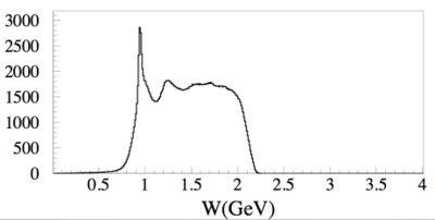
The gaussian shape of the [math]\Delta[/math] "bump" shows how this state does not have a well defined energy but rather can be created over a range [math]\Delta E[/math] of energies. The "Width" ([math]\Gamma[/math]) of an exclusive distribution determined a fit to a Breit Wigner function like
- [math]f(E) \sim \frac{1}{(E^2-M^2)^2-M^2 \Gamma^2}[/math]
where
- [math]E=[/math] Center of Mass energy
- [math]M=[/math] Mass of the resonance
- [math]\Gamma =[/math] resonance's Width
Fermi's Golden Rule
[1]Forest_FermiGoldenRule_Notes
Forest_NucPhys_I


