Plotting Different Frames
Jump to navigation
Jump to search
We can define different arrays to collect the coordinates in the different frames using a passive transformation. Assuming that the intersection of the ellipse and sense wires is in the y-x plane, we will have a positive rotation,
rFromYtoX = ( {
    {Cos[6 \[Degree]], -Sin[6 \[Degree]], 0},
    {Sin[6 \[Degree]], Cos[6 \[Degree]], 0},
    {0, 0, 1}
   } );
rFromXtoY = ( {
    {Cos[6 \[Degree]], Sin[6 \[Degree]], 0},
    {-Sin[6 \[Degree]], Cos[6 \[Degree]], 0},
    {0, 0, 1}
   } );
yxPoints = constant\[Theta];
constant\[Theta]yx = constant\[Theta];
constant\[Theta]yxRotated = constant\[Theta];
constant\[Theta]xyz = constant\[Theta];
constant\[Theta]xyzRotated = constant\[Theta];

RowLengths = Table[{Nothing}, {i, 1, 36}];
For[rows = 1, rows < 37, rows++,
  RowLengths[[rows]] = Length[constant\[Theta][[rows]]];
  For[columns = 1, columns < RowLengths[[rows]] + 1, columns++,
   \[Theta] = rows + 4;
   \[Phi] = constant\[Theta][[rows, columns, 1]];
   constant\[Theta]yx[[rows, columns]] = {y,
     Sqrt[a^2 (1 - y^2/b^2)] - \[CapitalDelta]a};
   constant\[Theta]xyz[[rows,
     columns]] = {constant\[Theta]yx[[rows, columns, 2]],
     constant\[Theta]yx[[rows, columns, 1]], 0};
   If[constant\[Theta][[rows, columns, 1]] < 0,
    constant\[Theta]yx[[rows, columns,
      1]] = -constant\[Theta]yx[[rows, columns, 1]];
    constant\[Theta]xyz[[rows, columns,
      2]] = -constant\[Theta]xyz[[rows, columns, 2]];
    ];
   constant\[Theta]xyzRotated[[rows, columns]] =
    rFromYtoX.{constant\[Theta]xyz[[rows, columns, 1]],
      constant\[Theta]xyz[[rows, columns, 2]],
      constant\[Theta]xyz[[rows, columns, 3]]};

   constant\[Theta]yxRotated[[rows,
     columns]] = {constant\[Theta]xyzRotated[[rows, columns, 2]],
     constant\[Theta]xyzRotated[[rows, columns, 1]]};
   yxPoints[[rows, columns]] = {y,
     Sqrt[a^2 (1 - y^2/b^2)] - \[CapitalDelta]a,
     constant\[Theta][[rows, columns, 1]],
     constant\[Theta][[rows, columns, 2]]};

   ]
  ];
ClearAll[\[Theta], \[Phi]];
DesiredyxPoints = Desiredconstant\[Theta];
Desiredconstant\[Theta]yx = Desiredconstant\[Theta];
Desiredconstant\[Theta]yxRotated = Desiredconstant\[Theta];
Desiredconstant\[Theta]xyz = Desiredconstant\[Theta];
Desiredconstant\[Theta]xyzRotated = Desiredconstant\[Theta];

DesiredRowLengths = Table[{Nothing}, {i, 1, 36}];
For[rows = 1, rows < 37, rows++,
  DesiredRowLengths[[rows]] =
   Length[Desiredconstant\[Theta][[rows]]];
  For[columns = 1, columns < DesiredRowLengths[[rows]] + 1,
   columns++,
   \[Theta] = rows + 4;
   \[Phi] = Desiredconstant\[Theta][[rows, columns, 1]];
   Desiredconstant\[Theta]yx[[rows, columns]] = {y,
     Sqrt[a^2 (1 - y^2/b^2)] - \[CapitalDelta]a};
   Desiredconstant\[Theta]xyz[[rows,
      columns]] = {Desiredconstant\[Theta]yx[[rows, columns, 2]],
     Desiredconstant\[Theta]yx[[rows, columns, 1]], 0};
   If[Desiredconstant\[Theta][[rows, columns, 1]] < 0,
    Desiredconstant\[Theta]yx[[rows, columns,
       1]] = -Desiredconstant\[Theta]yx[[rows, columns, 1]];
    Desiredconstant\[Theta]xyz[[rows, columns,
       2]] = -Desiredconstant\[Theta]xyz[[rows, columns, 2]];
    ];
   Desiredconstant\[Theta]xyzRotated[[rows, columns]] =
    rFromYtoX.{Desiredconstant\[Theta]xyz[[rows, columns, 1]],
      Desiredconstant\[Theta]xyz[[rows, columns, 2]],
      Desiredconstant\[Theta]xyz[[rows, columns, 3]]};

   Desiredconstant\[Theta]yxRotated[[rows,
      columns]] = {Desiredconstant\[Theta]xyzRotated[[rows, columns,
       2]], Desiredconstant\[Theta]xyzRotated[[rows, columns, 1]]};
   DesiredyxPoints[[rows, columns]] = {y,
     Sqrt[a^2 (1 - y^2/b^2)] - \[CapitalDelta]a,
     Desiredconstant\[Theta][[rows, columns, 1]],
     Desiredconstant\[Theta][[rows, columns, 2]]};

   ]
  ];
ClearAll[\[Theta], \[Phi]]
The parameter's range changes from the DC frame with 0<t<2, since
In the frame of the wires, the x axis no longer is aligned with the semi-major axis, therefore for in the DC frame
In[153]:= ClearAll[X, \[Theta]];
\[Theta] = 40;
X = X /. Solve[(X + \[CapitalDelta]a)^2/a^2 == 1 && X > 0, X]

Out[155]= {1.68318}
This gives the (x' , y')=(1.68318, 0) in the DC frame for
The slope m, with respect to x, is found as
Slope point form gives
SemiMajorAxisRotatedReverse =
  ContourPlot[X == -9.514 Y, {Y, -2, 2}, {X, 0, 1.8},
   Frame -> {True, True, False, False},
       PlotLabel ->
    "Right side limit of DC as a function of X and Y",
   FrameLabel -> {"y (meters)", "x (meters)"},
   ContourStyle -> Green,
       PlotLegends -> Automatic];
Graphing the frame of the sector and the wires within the sector,
DataXY = Table[
ListPlot[{constant\[Theta]yx[[i]]}, PlotStyle -> Black,
AxesLabel -> {"y", "x"},
PlotLabel ->
"DC Wire for Constant \[Theta] as a Function of \[Phi]"], {i, 1,
36}];
DataXYRotated =
Table[ListPlot[{constant\[Theta]yxRotated[[i]]}, PlotStyle -> Black,
AxesLabel -> {"y'", "x'"},
PlotLabel ->
"DC Wire for Constant \[Theta] as a Function of \[Phi]"],
{i, 1, 36}];
DesiredDataXY =
Table[ListPlot[{Desiredconstant\[Theta]yx[[i]]}, PlotStyle -> Black,
AxesLabel -> {"y", "x"},
PlotLabel ->
"DC Wire for Constant \[Theta] as a Function of \[Phi]"], {i, 1,
36}];
DesiredDataXYRotated =
Table[ListPlot[{Desiredconstant\[Theta]yxRotated[[i]]},
PlotStyle -> Black, AxesLabel -> {"y'", "x'"},
PlotLabel ->
"DC Wire for Constant \[Theta] as a Function of \[Phi]"],
{i, 1, 36}];
ClearAll[\[Theta]];
\[Theta] = 40;
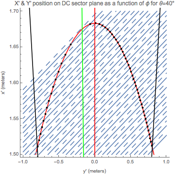
ellipse40 =
ContourPlot[(x + \[CapitalDelta]a)^2/a^2 + y^2/b^2 == 1, {y, -1,
1}, {x, 1.5, 1.7}, Frame -> {True, True, False, False},
PlotLabel ->
"X' & Y' position on DC sector plane as a function of \[Phi] for \
\[Theta]=40\[Degree]", FrameLabel -> {"y' (meters)", "x' (meters)"},
ContourStyle -> Red, PlotLegends -> Automatic];
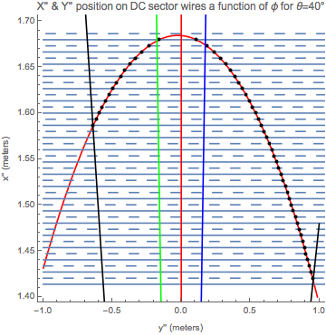
ellipse40Rotated =
ContourPlot[(X Cos[6 \[Degree]] +
Y Sin[6 \[Degree]] + \[CapitalDelta]a)^2/
a^2 + (-X Sin[6 \[Degree]] + Y Cos[6 \[Degree]])^2/b^2 ==
1, {Y, -1, 1}, {X, 1.4, 1.7}, Frame -> {True, True, False, False},
PlotLabel ->
"X'' & Y'' position on DC sector wires a function of \[Phi] for \
\[Theta]=40\[Degree]", FrameLabel -> {"y'' (meters)", "x'' (meters)"},
ContourStyle -> Red, PlotLegends -> Automatic];
Show[ellipse40,
Table[ContourPlot[
xWire == Tan[6 \[Degree]] yWire + x0forWires[number], {yWire, -1,
1}, {xWire, 1.5, 1.7},
FrameLabel -> {"y(meters)", "x(meters)"}], {number, 89, 109}],
Table[ContourPlot[
xWire ==
Tan[6 \[Degree]] yWire + x0forWireMiddles[number2], {yWire, -1,
1}, {xWire, 1.5, 1.7},
ContourStyle -> {Dashing[Large]}], {number2, 89, 109}],
DataXY[[36]],
DesiredDataXY[[36]], left, right, SemiMajorAxis, \
SemiMajorAxisRotatedReverse]
Show[ellipse40Rotated,
Table[ContourPlot[
xWire == Cos[6 \[Degree]] x0forWires[number], {yWire, -1,
1.2}, {xWire, 1.4, 1.7},
FrameLabel -> {"y(meters)", "x(meters)"}], {number, 89, 109}],
Table[ContourPlot[
xWire == Cos[6 \[Degree]] x0forWireMiddles[number2], {yWire, -1,
1.2}, {xWire, 1.4, 1.7},
ContourStyle -> {Dashing[Large]}], {number2, 89, 109}],
DataXYRotated[[36]],
DesiredDataXYRotated[[36]], rightRotated, leftRotated, \
SemiMajorAxisRotated, SemiMajorAxis, SemiMajorAxisRotatedReverse]
ClearAll[\[Theta]];

