|
|
| (30 intermediate revisions by 2 users not shown) |
| Line 8: |
Line 8: |
| | | | |
| | =Can one use plant material to measure the provenance of selenium?= | | =Can one use plant material to measure the provenance of selenium?= |
| | + | |
| | + | [[Se_Overview_PrevMeas]] |
| | | | |
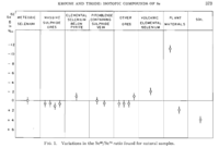
| | As shown in the Figure below, the Se-82/Se-76 ratio varies from -1.2% to +0.2% for plant materials but remains relatively constant for other materials. The variations in plant material has been described as being due to differences in the bacteria residing in the plant. The question to investigate is whether or not these variations in the concentration can be used to determine the provenance of the sample. | | As shown in the Figure below, the Se-82/Se-76 ratio varies from -1.2% to +0.2% for plant materials but remains relatively constant for other materials. The variations in plant material has been described as being due to differences in the bacteria residing in the plant. The question to investigate is whether or not these variations in the concentration can be used to determine the provenance of the sample. |
| Line 67: |
Line 69: |
| | | | |
| | =Experiments= | | =Experiments= |
| | + | |
| | + | ==[[PAA_Selenium_ActivityCalc]]== |
| | + | |
| | [[PAA Selenium/Soil Experiments]] | | [[PAA Selenium/Soil Experiments]] |
| | | | |
| | + | [[LB Se PAA Horse Feed Experiment]] |
| | | | |
| | + | ==Background Signals== |
| | + | [[PAA_BackGrd_Det_A]] |
| | | | |
| | ==Nickel Normalization== | | ==Nickel Normalization== |
| | [[LB PAA Nickel Investigation]] | | [[LB PAA Nickel Investigation]] |
| − |
| |
| − | ==Chlorine==
| |
| − |
| |
| − | It looks like Cl-35 is abundant as you see photon energies of 146 keV and 2127 keV (you can barely see 1176 keV) from Cl-34's decay (neutron knocked out of Cl-35).
| |
| − |
| |
| − | The half life is 32 minutes.
| |
| − |
| |
| − | Should check the half life from the run AccOnAlInDetASe-AinDetD_001.root using the calibration
| |
| − |
| |
| − | MPA->Draw("0.18063+0.960133*evt.Chan>> SeRun_008(8000,0.5,8000.5)","evt.ADCid==3");
| |
| − |
| |
| − | == Irradiation of Horse Mineral Supplement==
| |
| − |
| |
| − | Below is the EMSL report for the horse feed sample.
| |
| − | https://wiki.iac.isu.edu/index.php/File:EMSL_Report_Horse_Feed.pdf
| |
| − |
| |
| − | === Chlorine is a dominant signal===
| |
| − |
| |
| − |
| |
| − | First, look at the peak around 146 keV
| |
| − | [[File:146_keV.png | 200 px]]
| |
| − |
| |
| − | Next I plotted the counts as a function of time to get an exponentially decaying graph. When doing an exponential fit here, the parameter "b" given by root will be the decay constant.
| |
| − |
| |
| − | [[ File:Chlorine.png | 200 px]]
| |
| − |
| |
| − | Root gives a half life of 32.9508 +/- 0.01 minutes
| |
| − |
| |
| − |
| |
| − | Now do the same for the 2127 keV line
| |
| − | [[File:2127_keV.png | 200 px]]
| |
| − |
| |
| − | Here are the counts plotted as a function of time
| |
| − | [[File:2127.png | 200 px ]]
| |
| − |
| |
| − | Root gives a half life of 35.3962 +/- 0.2 minutes
| |
| − |
| |
| − | === Potassium is a potential signal ===
| |
| − |
| |
| − | Looking at the spectrum for the fast irradiation sample, there are 2 prominent lines that could be from 38-K. The mechanism would be a single neutron knockout from a stable 39-K nucleus. The two most dominant energies of the three for 38-K are 2167 keV and 3936 keV and the half life is 7.63 minutes. Below is a fit to the energy spectrum histogram
| |
| − |
| |
| − | [[File:2168_peak.png | 200 px]]
| |
| − |
| |
| − | Now check the half life
| |
| − |
| |
| − |
| |
| − | [[File:2167.png | 200 px]]
| |
| − |
| |
| − | Root gives a half life of 8.03 +/- 0.02 minutes
| |
| − |
| |
| − | Next check the 3936 peak
| |
| − |
| |
| − | [[File: 3937_Peak.png | 200 px ]]
| |
| − |
| |
| − | and check the half life
| |
| − |
| |
| − | [[File: 3936_keV_halflife.png | 200 px ]]
| |
| − |
| |
| − | Root gives a value for b = - 1.14372x10^(-3), which in turn gives a half life of 10.1 minutes
| |
| − |
| |
| − | It seems very possible that 38-K could be in the sample of horse feed.
| |
| | | | |
| | == First Observation of Se lines== | | == First Observation of Se lines== |
| Line 148: |
Line 95: |
| | ==IAC Detector Efficiencies == | | ==IAC Detector Efficiencies == |
| | | | |
| − | Below is the runlist for finding the efficiency of the detector at position R
| + | [[LB PAA IAC Detector Efficiencies]] |
| − | | |
| − | | |
| − | {| border="3" cellpadding="5" cellspacing="0"
| |
| − | | Source || Serial # || Reference Date || Activity || Start || Stop || Live
| |
| − | |-
| |
| − | | Na-22 || 129743 || 7-01-08 || 9.427 microCi || 15:49 || 16:19 || 1796.803
| |
| − | |-
| |
| − | | Cs-137 || 129793 || 7-01-08 || 1.006 microCi || 14:25 || 14:56 || 1879.606
| |
| − | |-
| |
| − | | Mn-54 || 129807 || 7-01-08 || 11.77 microCi || 15:00 || 15:30 || 1793.420
| |
| − | |-
| |
| − | | Co-60 || 129740 || 7-01-08 || 10.42 microCi || 15:33 || 15:43 || 569.725
| |
| − | |-
| |
| − | |}
| |
| − | | |
| − | Below are the theoretical calculations for the theoretical decay frequencies
| |
| − | | |
| − | Na-22, 9.427micro Ci on July 1, 2008, half life 2.602 +/- 0.002 years, 99.937% for 1274.52 and 178.8 for 511 line , activity in March 31, 2016 =1.196micro Ci
| |
| − | := <math>\left (0.99937 \right )\left ( 1.196 \times 10^{-6} \mbox{Ci} \right) \left (\frac{ (3.7 \times 10^{10} \mbox{Hz}}{\mbox{Ci}} \right)= 44,224 Hz </math> for the 1274 line
| |
| − | | |
| − | := <math>\left (1.788 \right )\left ( 1.196 \times 10^{-6} \mbox{Ci} \right) \left (\frac{ (3.7 \times 10^{10} \mbox{Hz}}{\mbox{Ci}} \right)= 79122.6 Hz </math> for the 511 line
| |
| − | | |
| − | Cs-137, 661.660 line, 85.21% * 1.066micro Ci on July 1, 2008, half life 30.0 +/- 0.2 yrs, March 31, 2016 activity = 0.891micro Ci expected rate for 661 line
| |
| − | | |
| − | := <math>\left (0.8521 \right )\left ( 0.891 \times 10^{-6} \mbox{Ci} \right) \left (\frac{ (3.7 \times 10^{10} \mbox{Hz}}{\mbox{Ci}} \right)= 28091.2 Hz </math>
| |
| − | | |
| − | Mn-54, 11.77 microCi on July 1, 2008, half life =312.20 +/- 0.07 days, 99.975% intensity on 834.826 , March 31, 2016 activity =0.02328micro Ci
| |
| − | | |
| − | := <math>\left (0.99975 \right )\left ( 0.02328 \times 10^{-6} \mbox{Ci} \right) \left (\frac{ (3.7 \times 10^{10} \mbox{Hz}}{\mbox{Ci}} \right)= 861.1 Hz </math> for the 834 line
| |
| − | | |
| − | | |
| − | Co-60, 10.42micro Ci July 1, 2008, half life 5.271 +/- 0.001 years, 99.0 % for 1173.237 and 99.9824 % for 1332.501, March 31, 2016 activity=3.759micro Ci
| |
| − | | |
| − | | |
| − | := <math>\left (0.99 \right )\left ( 3.759 \times 10^{-6} \mbox{Ci} \right) \left (\frac{ (3.7 \times 10^{10} \mbox{Hz}}{\mbox{Ci}} \right)= 137692.17 Hz </math> for the 1173 line
| |
| − | | |
| − | | |
| − | := <math>\left (0.999824 \right )\left ( 3.759 \times 10^{-6} \mbox{Ci} \right) \left (\frac{ (3.7 \times 10^{10} \mbox{Hz}}{\mbox{Ci}} \right)= 139058.52 Hz </math> for the 1332 line
| |
| − | | |
| − | | |
| − | Below is a table where the actual efficiency will be calculated for position R (farthest position).
| |
| − | | |
| − | {| border="3" cellpadding="5" cellspacing="0"
| |
| − | | Run || Source || Energy (keV) || Expected Rate (Hz) || HpGe Rate (Hz) || HpGe Det D Efficiency (%)
| |
| − | |-
| |
| − | | Eff_003 || Na-22 || 511 || 79122.6 || (506:516) (4.309-0.065=4.244) || 0.005
| |
| − | |-
| |
| − | | Eff_005 || Cs-137 || 661.657 || 28091.2 ||(657:666)(1.105-0.02281=1.0821) ||0.004
| |
| − | |-
| |
| − | | Eff_006 || Mn-54 || 834.848 || 861.1 ||(830:839)(0.04037-0.009123=0.031247)||0.004
| |
| − | |-
| |
| − | | Eff_007 || Co-60 || 1173.228 || 137692 ||(1164:1182)(3.686-0.01939=3.67)||0.003
| |
| − | |-
| |
| − | | Eff_003 || Na-22 || 1274.537 || 44224 ||(1270:1279) (1.073-0.0057=1.0673)||0.002
| |
| − | |-
| |
| − | | Eff_007 || Co-60 || 1332.492 || 139058.52 ||(1328:1337)(3.283-0.05702=3.22598)|| 0.002
| |
| − | |}
| |
| − | | |
| − | Below is a runlist for position k
| |
| − | | |
| − | {| border="3" cellpadding="5" cellspacing="0"
| |
| − | | Source || Serial # || Reference Date || Activity || Start || Stop || Live
| |
| − | |-
| |
| − | | Na-22 || 129743 || 7-01-08 || 9.427 microCi || 14:54 || 15:01 || 434.087
| |
| − | |-
| |
| − | | Cs-137 || 129793 || 7-01-08 || 1.006 microCi || 15:48 || 15:55 || 413.925
| |
| − | |-
| |
| − | | Mn-54 || 129807 || 7-01-08 || 11.77 microCi || 15:28 || 15:40 || 705.186
| |
| − | |-
| |
| − | | Co-60 || 129740 || 7-01-08 || 10.42 microCi || 15:41 || 15:47 || 346.092
| |
| − | |-
| |
| − | |}
| |
| − | | |
| − | Below are the theoretical decay frequencies
| |
| − | | |
| − | Na-22, 9.427micro Ci on July 1, 2008, half life 2.602 +/- 0.002 years, 99.937% for 1274.52 and 178.8 for 511 line , activity in April 14, 2016 =1.183micro Ci
| |
| − | := <math>\left (0.99937 \right )\left ( 1.183 \times 10^{-6} \mbox{Ci} \right) \left (\frac{ (3.7 \times 10^{10} \mbox{Hz}}{\mbox{Ci}} \right)= 43743.4 Hz </math> for the 1274 line
| |
| − | | |
| − | := <math>\left (1.788 \right )\left ( 1.183 \times 10^{-6} \mbox{Ci} \right) \left (\frac{ (3.7 \times 10^{10} \mbox{Hz}}{\mbox{Ci}} \right)= 78262.5 Hz </math> for the 511 line
| |
| − | | |
| − | Cs-137, 661.660 line, 85.21% * 1.066micro Ci on July 1, 2008, half life 30.0 +/- 0.2 yrs, April 14, 2016 activity =0.890 micro Ci expected rate for 661 line
| |
| − | | |
| − | := <math>\left (0.8521 \right )\left ( 0.890 \times 10^{-6} \mbox{Ci} \right) \left (\frac{ (3.7 \times 10^{10} \mbox{Hz}}{\mbox{Ci}} \right)= 28059.7 Hz </math>
| |
| − | | |
| − | Mn-54, 11.77 on July 1, 2008, half life =312.20 +/- 0.07 days, 99.975% intensity on 834.826 , April 14, 2016 activity =0.02251micro Ci
| |
| − | | |
| − | := <math>\left (0.99975 \right )\left ( 0.02251 \times 10^{-6} \mbox{Ci} \right) \left (\frac{ (3.7 \times 10^{10} \mbox{Hz}}{\mbox{Ci}} \right)= 830.79 Hz </math> for the 834 line
| |
| − | | |
| − | | |
| − | Co-60, 10.42micro Ci July 1, 2008, half life 5.271 +/- 0.001 years, 99.0 % for 1173.237 and 99.9824 % for 1332.501, April 14, 2016 activity=3.74micro Ci
| |
| − | | |
| − | | |
| − | := <math>\left (0.99 \right )\left ( 3.74 \times 10^{-6} \mbox{Ci} \right) \left (\frac{ (3.7 \times 10^{10} \mbox{Hz}}{\mbox{Ci}} \right)= 136996.2 Hz </math> for the 1173 line
| |
| − | | |
| − | | |
| − | := <math>\left (0.999824 \right )\left ( 3.74 \times 10^{-6} \mbox{Ci} \right) \left (\frac{ (3.7 \times 10^{10} \mbox{Hz}}{\mbox{Ci}} \right)= 138355.6 Hz </math> for the 1332 line
| |
| − | | |
| − | Below are the actual efficiencies for position k
| |
| − | | |
| − | {| border="3" cellpadding="5" cellspacing="0"
| |
| − | | Run || Source || Energy (keV) || Expected Rate (Hz) || HpGe Rate (Hz) || HpGe Det D Efficiency (%)
| |
| − | |-
| |
| − | | Eff_k_002 || Na-22 || 511 || 79122.6 || (506:516)(49.21-0.6272=48.58) || 0.06
| |
| − | |-
| |
| − | | Eff_k_006 || Cs-137 || 661.657 || 28091.2 ||(657:666)(12.86-0.02281=12.837) ||0.05
| |
| − | |-
| |
| − | | Eff_k_004 || Mn-54 || 834.848 || 861.1 ||(830:839)(0.3204-0.009123=0.311)||0.04
| |
| − | |-
| |
| − | | Eff_k_005 || Co-60 || 1173.228 || 137692 ||(1164:1182)(42.39-0.02053=42.369)||0.03
| |
| − | |-
| |
| − | | Eff_k_002 || Na-22 || 1274.537 || 44224 ||(1270:1279) (12.53-0.005702)=12.52||0.03
| |
| − | |-
| |
| − | | Eff_k_005 || Co-60 || 1332.492 || 139058.52 ||(1328:1337)(35.94-0.005072)|| 0.03
| |
| − | |}
| |
| − | | |
| − | Below is a runlist for position C
| |
| − | | |
| − | {| border="3" cellpadding="5" cellspacing="0"
| |
| − | | Source || Serial # || Reference Date || Activity || Start || Stop || Live
| |
| − | |-
| |
| − | | Na-22 || 129742 || 7-01-08 || 1.146 microCi || 12:55 || 12:57 || 129.782
| |
| − | |-
| |
| − | | Cs-137 || 129793 || 7-01-08 || 1.006 microCi || 13:02 || 13:04 || 123.818
| |
| − | |-
| |
| − | | Mn-54 || 129806 || 7-01-08 || 1.226 microCi || 13:11 || 13:21 || 613.754
| |
| − | |-
| |
| − | | Co-60 || 129739 || 7-01-08 || 1.082 microCi || 13:08 || 13:09 || 103.599
| |
| − | |-
| |
| − | |}
| |
| − | | |
| − | Below are the calculations for the theoretical frequencies
| |
| − | | |
| − | Na-22, 9.427micro Ci on July 1, 2008, half life 2.602 +/- 0.002 years, 99.937% for 1274.52 and 178.8 for 511 line , activity in May 5, 2016 =1.196micro Ci
| |
| − | := <math>\left (0.99937 \right )\left ( 0.14 \times 10^{-6} \mbox{Ci} \right) \left (\frac{ (3.7 \times 10^{10} \mbox{Hz}}{\mbox{Ci}} \right)= 5176.7 Hz </math> for the 1274 line
| |
| − | | |
| − | := <math>\left (1.788 \right )\left ( 0.14 \times 10^{-6} \mbox{Ci} \right) \left (\frac{ (3.7 \times 10^{10} \mbox{Hz}}{\mbox{Ci}} \right)= 9261.8 Hz </math> for the 511 line
| |
| − | | |
| − | Cs-137, 661.660 line, 85.21% * 1.066micro Ci on July 1, 2008, half life 30.0 +/- 0.2 yrs, May 5, 2016 activity = 0.89micro Ci expected rate for 661 line
| |
| − | | |
| − | := <math>\left (0.8521 \right )\left ( 0.891 \times 10^{-6} \mbox{Ci} \right) \left (\frac{ (3.7 \times 10^{10} \mbox{Hz}}{\mbox{Ci}} \right)= 28059.7 Hz </math>
| |
| − | | |
| − | Mn-54, 1.226 microCi on July 1, 2008, half life =312.20 +/- 0.07 days, 99.975% intensity on 834.826 , May 5, 2016 activity =0.002micro Ci
| |
| − | | |
| − | := <math>\left (0.99975 \right )\left ( 0.002 \times 10^{-6} \mbox{Ci} \right) \left (\frac{ (3.7 \times 10^{10} \mbox{Hz}}{\mbox{Ci}} \right)= 73.98 Hz </math> for the 834 line
| |
| − | | |
| − | | |
| − | Co-60, 1.082micro Ci July 1, 2008, half life 5.271 +/- 0.001 years, 99.0 % for 1173.237 and 99.9824 % for 1332.501, May 5, 2016 activity=0.39micro Ci
| |
| − | | |
| − | | |
| − | := <math>\left (0.99 \right )\left ( 0.39 \times 10^{-6} \mbox{Ci} \right) \left (\frac{ (3.7 \times 10^{10} \mbox{Hz}}{\mbox{Ci}} \right)= 14285.7 Hz </math> for the 1173 line
| |
| − | | |
| − | | |
| − | := <math>\left (0.999824 \right )\left ( 0.39 \times 10^{-6} \mbox{Ci} \right) \left (\frac{ (3.7 \times 10^{10} \mbox{Hz}}{\mbox{Ci}} \right)= 14427.5 Hz </math> for the 1332 line
| |
| − | | |
| − | Below is a table with the calculated efficiencies
| |
| − | | |
| − | {| border="3" cellpadding="5" cellspacing="0"
| |
| − | | Run || Source || Energy (keV) || Expected Rate (Hz) || HpGe Rate (Hz) || HpGe Det D Efficiency (%)
| |
| − | |-
| |
| − | | Eff_C_001 || Na-22 || 511 || 9261.8 || (506:516) (45.65-0.065=45.585) || 0.5
| |
| − | |-
| |
| − | | Eff_C_002 || Cs-137 || 661.657 || 28059.7 ||(657:666)(101.7-0.02281=101.67) || 0.4
| |
| − | |-
| |
| − | | Eff_C_004 || Mn-54 || 834.848 || 73.98 ||(830:839)(0.2704-0.009123=0.2612)||0.4
| |
| − | |-
| |
| − | | Eff_C_003 || Co-60 || 1173 || 14285.7 ||(1164:1182)(34.24-0.01939=34.22)||0.2
| |
| − | |-
| |
| − | | Eff_C_001 || Na-22 || 1274.537 || 5176.7 ||(1270:1279) (11.15-0.0057=11.14)||0.2
| |
| − | |-
| |
| − | | Eff_C_003 || Co-60 || 1332.492 || 14427.5 ||(1328:1337)(28.05-0.05702=27.99)|| 0.2
| |
| − | |}
| |
| − | | |
| − | =Run List=
| |
| | | | |
| − | {| border="3" cellpadding="5" cellspacing="0"
| + | ==IAC Detector Calibrations== |
| − | | Date || Time elapsed (Seconds) || Sample || Document Title || Start || Stop || Real || Live || Position
| |
| − | |-
| |
| − | | 04-01-16 || 2.16x10^6 || Se_B || Se_B_002 || 15:55 || 09:15 || 235989.882 || 235687.660 || k
| |
| − | |-
| |
| − | | 04-06-16 || 2.592x10^6 || Se_B || Se_B_003 || 12:57 || Interrupted || computer || crash || k
| |
| − | |-
| |
| − | | 04-14-16 || 3.283x10^6 || Se_B || Se_B_005 || 15:57 || 09:37 || 63581.784 || 63509.895||k
| |
| − | |-
| |
| − | | 04-15-16 || 3.37x10^6 || Sample D || Sample_D_001 || 14:47 || 08:23 || 236172.264 || 236173.271||k
| |
| − | |-
| |
| − | | 04-19-16 || 3.715x10^6 || Sample B || Sample_B_001 ||15:31||15:18 || 85634.862 || 85624.090||k
| |
| − | |-
| |
| − | | 4-20-16 || 3.802x10^6 || Sample C || Sample_C_001 ||15:22||10:19 || 68253.774 || 68232.238||k
| |
| − | |-
| |
| − | | 04-21-16 || 3.888x10^6 || Sample A || Sample_A_001 || 10:22 || 10:37 || 87292.409 || 87268.114||k
| |
| − | |-
| |
| − | |04-25-16 || 4.234x10^6 || Sample E || Sample_E_001 || 11:36 || 10:03 || 80822.406 || 80795.679||k
| |
| − | |-
| |
| − | |04-26-16 || 4.32x10^6 || Se_B || Se_B_008 || 10:06 || 10:29 || 87784.755 || 87664.070 || k
| |
| − | |-
| |
| − | |05-05-16 || 5.098x10^6 || Sample A || Sample_A_002 || 13:31 || 14:30 || 3605.507 || 3602.925 || c
| |
| − | |-
| |
| − | |05-05-16 || 5.098x10^6 || Sample B || Sample_B_002 || 14:34 || 15:26 || 3114.244 || 3112.620 || c
| |
| − | |-
| |
| − | |05-05-16 || 5.098x10^6 || Sample C || Sample_C_002 || 15:28 || 10:57 || 70124.788 || 70044.470 || c
| |
| − | |-
| |
| − | | 05-06-16 ||5.184x10^6|| Sample D || Sample_D_002 || 10:59 || 15:34 || 16516.898 || 16512.570||c
| |
| − | |-
| |
| − | |05-06-16 || 5.184x10^6 || Sample E || Sample_E_004 || 15:37 || 16:18 || 261654.225 || 261344.308 || c
| |
| − | |-
| |
| − | |05-09-16 || 5.443x10^6 || Se B|| Se_B_012 || 16:20 || 11:08||67157.101||66660.298 || c
| |
| − | |-
| |
| − | |05-10-16 || 5.5296x10^6 || Sample A || Sample_A_004 || 11:03 || 15:19 || 15379.475 || 15363.017 || c
| |
| − | |-
| |
| − | |05-10-16 || 5.5296x10^6 || Sample B || Sample_B_004 || 15:22:04 || 11:43 || 73256.181 || 73220.324 || c
| |
| − | |-
| |
| − | |05-16-16 || 6.048x10^6 || Sample C || Sample_C_004 || 16:33 || 08:19 || 56758.980 || 56711.121 || c
| |
| − | |-
| |
| − | |05-18-16 || 6.2208x10^6 || Sample D || Sample_D_006 || 08:44:21 || 14:05 || 19271.829 || 19266.929 || c
| |
| − | |-
| |
| − | |05-18-16 || 6.2208x10^6 || Sample E || Sample_E_006 || 14:08 || 08:06 || 151108.258 || 150955.915 || c
| |
| − | |-
| |
| − | |05-20-16 || 6.3936x10^6 || Se_B || Se_B_014 || 08:08:47 || 08:44 || 261353.204 || 259621.655 || c
| |
| − | |-
| |
| − | |05-23-16 || 6.6528x10^6 || Sample A || Sample_A_006 || 08:48 || 13:49 || 18103.004 || 18091.523 || c
| |
| − | |-
| |
| − | |05-23-16 || 6.6528x10^6 || Sample B || Sample_B_006 || 13:52 || 13:24 || 84763.938 || 84696.083 || c
| |
| − | |-
| |
| − | |05-24-16 || 6.7392x10^6 || Sample C || Sample_C_006 || 13:28:28 || 10:28 || 75571.716 || 75502.871 || c
| |
| − | |-
| |
| − | |05-31-16 || 7.344x10^6 || Sample B || Sample_B_008 || 08:57:22 || 08:55 || 86282.861 || 86237.392 || c
| |
| − | |-
| |
| − | |06-01-16 || 7.4304x10^6 || Sample C || Sample_C_008 || 08:58:39 || 13:31 || 102739.504 || 102647.471 || c
| |
| − | |-
| |
| − | |06-02-16 || 7.5168x10^6 || Sample D || Sample_D_010 || 13:33 || 08:41 || 68915.044 || 68898.246 || c
| |
| − | |}
| |
| | | | |
| − | ==[[SeRun_01-11-16]]==
| + | [[LB April DetB DetA Calibration]] |
| − | ==[[LB March 2017 Runlist]]==
| |
| | | | |
| − | ==[[SeRun_03-07-16]]== | + | ==Runlists== |
| | + | [[LB PAA Runlist 4/01/16 - 06/02/16]] |
| | | | |
| − | ==[[SeRun_02-13-17]]==
| + | [[LB March 2017 Runlist]] |
| | | | |
| − | ==[[LB IAC Radiator Specs]]==
| + | [[LB_May_2017_Irradiation_Day]] |
| − | | |
| − | ==[[LB Rotating Sample Holder]]==
| |
| − | ==[[LB April DetB DetA Calibration]]==
| |
| | | | |
| | =Data Analysis= | | =Data Analysis= |
| | | | |
| − | ==Pure Se Sample==
| |
| − |
| |
| − | ===Observed lines===
| |
| | | | |
| | [[LB_Feb2017_Se_Investigations]] | | [[LB_Feb2017_Se_Investigations]] |
| − |
| |
| − | ===Estimate of Se-79 activity===
| |
| − |
| |
| − | Using known efficiency to extrapolate initial activity
| |
| − |
| |
| − | Use ratio with Nickel foil rate
| |
| − |
| |
| − | == Se spiked in Soil==
| |
| − |
| |
| − |
| |
| − |
| |
| − | Detection limit of Se in Soil
| |
| | | | |
| | =References= | | =References= |
Using PAA ro measure Selenium concentrations.
According to Krouse<ref name="Krous1962"> H.R. Krause and H.G. Thode,"Thermodynamic Properties and Geochemistry of Iosotopic Compounds of Selenium",.Can. J. Chem., vol 40, pg 367</ref>
, the fractional concentration of Se-82/Se-76 in plant material is observed to be less than from primordial (meteoric) concentrations by as much as 1.2%. Anaerobic bacteria are known to reduce selenates and senelites in biological systems. This may be the reason plant material has fractionation of selenium isotopes. They also observe excess concentrations of up to 0.4% in soil.
Plant material appears to detect environmental selenium.
Can one use plant material to measure the provenance of selenium?
Se_Overview_PrevMeas
As shown in the Figure below, the Se-82/Se-76 ratio varies from -1.2% to +0.2% for plant materials but remains relatively constant for other materials. The variations in plant material has been described as being due to differences in the bacteria residing in the plant. The question to investigate is whether or not these variations in the concentration can be used to determine the provenance of the sample.
Below is a table listing the natural abundances of Selenium
Natural abundance of selenium
| Isotope |
Abundance
|
| Se-74 |
0.86%
|
| Se-76 |
9.23%
|
| Se-77 |
7.60%
|
| Se-78 |
23.69%
|
| Se-80 |
49.80%
|
| Se-82 |
8.82%
|
Below are possible PAA reactions that may be used to observe specific Se isotopes
| Reaction |
Half-life |
Relative activity |
Gamma-rays, keV (BR)
|
| Se-74(gamma,n)Se-73 |
7.1 h |
1.5E-1 |
361 (100)
|
| Se-74(gamma,n)Se-73m |
39 m |
3.2 |
402 (4)
|
| Se-74(gamma,np)As-72 |
26 h |
1.0E-3 |
834 (100)
|
| Se-76(gamma,n)Se-75 |
120 d |
1.3E-2 |
265(29)
|
| Se-77(gamma,p)As-76 |
26.4 h |
4.4E-2 |
559(44)
|
| Se-78(gamma,p)As-77 |
38.8 h |
8.6E-2 |
239(2)
|
| Se-80(gamma,n)Se-79m |
3.9 m |
5.9 |
96(10)
|
| Se-80(gamma,np)As-78 |
1.5 h |
2.2E-2 |
614(54)
|
| Se-80(gamma,p)As-79 |
8.2 m |
1.3 |
96(9)
|
| Se-80(gamma,[math]a[/math]p)Ge-75 |
83 m |
2.8E-1 |
265(11)
|
Can one perform PAA measurements of Se-82 and Se-76?
Se_PAA_Reactions
Experiments
PAA Selenium/Soil Experiments
LB Se PAA Horse Feed Experiment
Background Signals
PAA_BackGrd_Det_A
Nickel Normalization
LB PAA Nickel Investigation
First Observation of Se lines
Using the 44 Machine at 7 kW power and 44 meV incident electron energy to produce a bremsstrahlung spectrum with a mean energy of 15 meV.
All runs lasting less than 214 seconds have time stamp that gives real time if you divide by clock frequency of 20 MHz. The first 32 bits are used for a real time measurement.
MDA and Se mass Calculations
LB MDA/Se Mass Calculations
IAC Detector Efficiencies
LB PAA IAC Detector Efficiencies
IAC Detector Calibrations
LB April DetB DetA Calibration
Runlists
LB PAA Runlist 4/01/16 - 06/02/16
LB March 2017 Runlist
LB_May_2017_Irradiation_Day
Data Analysis
LB_Feb2017_Se_Investigations
References
User_talk:Brenleyt
<references/>
File:Krouse CanJournChem 40 1962 p367.pdf
Goryachev, A. M., & Zalesnyy, G. N. (n.d.). The studying of the photoneutron reactions cross sections in the region of the giant dipole resonance in zinc, germanium, selenium, and strontium isotopes. Retrieved September 16, 2016, from http://www-nds.indcentre.org.in/exfor/servlet/X4sSearch5?EntryID=220070
Goryachev, B. I., Ishkhanov, B. S., Kapitonov, I. M., Piskarev, I. M., Piskarev, V. G., & Piskarev, O. P. (n.d.). Giant Dipole Resonance on Ni Isotopes. Retrieved October 26, 2016, from http://www-nds.indcentre.org.in/exfor/servlet/X4sGetSubent?reqx=119235&subID=220597006&plus=1
Handbook on Photonuclear data for applications, cross sections, and spectra. (2000, October). Retrieved November 4, 2016, from http://www-pub.iaea.org/MTCD/Publications/PDF/te_1178_prn.pdf
MSDS
Selenium shot, amorphous, 2-6 mm, Puratronic, 99.999% Alfa Aesar product # 10603 File:AlphaAesarSelenium MDSD.pdf
Informative links
http://www.deq.idaho.gov/regional-offices-issues/pocatello/southeast-idaho-phosphate-mining/southeast-idaho-selenium-investigations/
https://inldigitallibrary.inl.gov/sti/3169894.pdf
http://giscenter.isu.edu/research/Techpg/sisp/index.htm
PAA_Research
