|
|
| (48 intermediate revisions by the same user not shown) |
| Line 1: |
Line 1: |
| | | | |
| − | <center><math>\textbf{Navigation}</math></center> | + | <center><math>\underline{\textbf{Navigation}}</math></center> |
| | | | |
| | <center> | | <center> |
| Line 27: |
Line 27: |
| | | | |
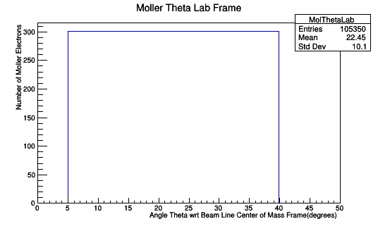
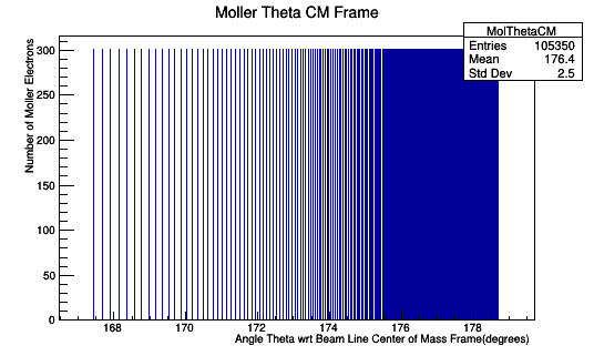
| | =LUND File Output= | | =LUND File Output= |
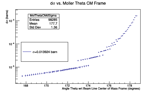
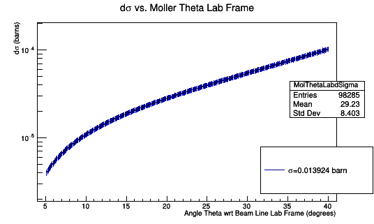
| − | | + | Uniform spacing in Lab frame, not in CM frame. |
| − | 0.1 degree spacing in the Lab frame. CM Frame is not evenly spaced. | + | ==0.1 degree spacing for θ in the Lab frame== |
| | | | |
| | | | |
| | [[File:MolThetaLab_LUND_DC_limits.png]][[File:MolThetaCM_LUND_DC_limits.png]] | | [[File:MolThetaLab_LUND_DC_limits.png]][[File:MolThetaCM_LUND_DC_limits.png]] |
| | | | |
| − | Applying the weight
| + | ==0.05 degree spacing for θ in the Lab frame== |
| − | | |
| − | [[File:MolThetaLab_DClimits_integral.png]][[File:CosMolThetaLab_weightedDClimits.png]]
| |
| − | | |
| − | | |
| − | [[File:MolThetaCM_DClimits_weighted_rebin_integral.png]][[File:CosMolThetaCM_weightedDClimits.png]]
| |
| − | | |
| − | | |
| − | Looking at the angles and the associated weight, we can find the sums
| |
| − | | |
| − | [[Once_Angles_and_weight]]=3399.930890560805437
| |
| − | | |
| − | [[Total_Angles_and_weight]]=1023379.198058736044914
| |
| − | | |
| − | | |
| − | Checking with Mathematica
| |
| − | | |
| − | [[File:CrossSectionMathematica1.png]]
| |
| − | | |
| − | | |
| − | "Integrating" with Cosine term
| |
| − | | |
| − | [[File:CrossSectionMathematica2.png]]
| |
| | | | |
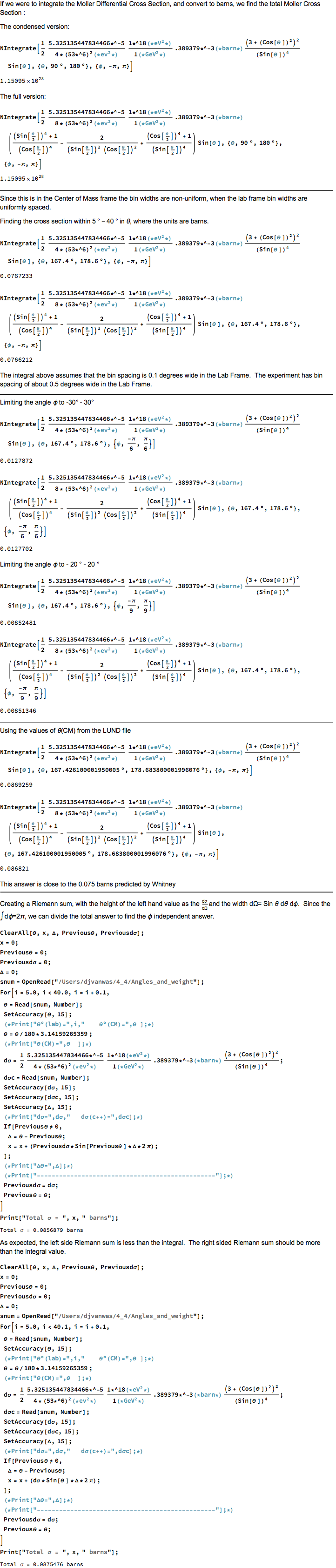
| | =Finding the Cross Section= | | =Finding the Cross Section= |
| − | | + | ==Total cross section over φ== |
| | [[File:CrossSectionMathematicaProof.png]] | | [[File:CrossSectionMathematicaProof.png]] |
| | | | |
| | + | ==Total cross section over DC limits== |
| | | | |
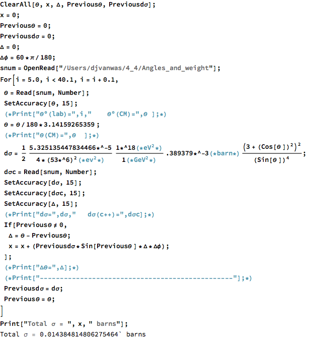
| − | Performing a Riemann sum for <math>-30^{\circ} \lt \phi \lt 30^{\circ}</math>
| |
| − |
| |
| − |
| |
| − | [[File:CrossSection60deg.png]]
| |
| − |
| |
| − |
| |
| − |
| |
| − | The cross section should be equal between both frames since the number of particles is an invariant. The differential cross section must differ between frames since the solid angle does vary.
| |
| − |
| |
| − | <center><math>\sigma_{(CM)}=\sigma{(Lab)}</math></center>
| |
| − |
| |
| − |
| |
| − | <center><math>\frac{d\sigma}{d\Omega}_{(CM)} d\Omega_{(CM)}=\frac{d\sigma}{d\Omega}_{(Lab)} d\Omega_{(Lab)}</math></center>
| |
| − |
| |
| − |
| |
| − |
| |
| − |
| |
| − | <center><math>\frac{d\sigma}{d\Omega}_{(CM)} \sin \theta_{(CM)}\ d\theta_{(CM)}\ d\phi=\frac{d\sigma}{d\Omega}_{(Lab)} \sin \theta_{(Lab)}\ d\theta_{(Lab)}\ d\phi</math></center>
| |
| − |
| |
| − |
| |
| − | <center><math>\rightarrow \frac{d\sigma}{d\Omega}_{(Lab)}=\frac{d\sigma}{d\Omega}_{(CM)} \frac{\sin \theta_{(CM)}\ d\theta_{(CM)}\ d\phi}{ \sin \theta_{(Lab)}\ d\theta_{(Lab)}\ d\phi}</math></center>
| |
| − |
| |
| − |
| |
| − |
| |
| − | <center><math>\rightarrow d\sigma_{(Lab)}=\frac{d\sigma}{d\Omega}_{(CM)} \frac{\sin \theta_{(CM)}\ d\theta_{(CM)}\ d\phi}{ \sin \theta_{(Lab)}\ d\theta_{(Lab)}\ d\phi}\sin \theta_{(Lab)} d\theta_{(Lab)}\ d\phi</math></center>
| |
| − |
| |
| − |
| |
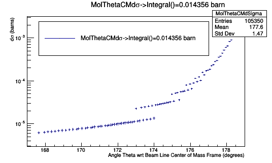
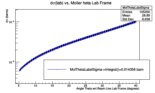
| − | [[File:MolThetaCMdsigmaIntegral.png]][[File:MolThetaLabdSigmaIntegral.png]]
| |
| − |
| |
| − | [[File:AssociatedWeights2.png]][[File:dSigmaCMLab.png]]
| |
| − |
| |
| − | ==Adjust for DC Sector 1 Limits==
| |
| − |
| |
| − | [[File:IntegralDCLimitsdSigmaCM.png]][[File:IntegralDCLimitsdSigmaLab.png]]
| |
| − |
| |
| − | =GEMC Cross Section=
| |
| − |
| |
| − |
| |
| − | Only taking GEMC hits in Sector 1 with Track ID of the mother of the FP equal to zero:
| |
| − |
| |
| − | [[File:DSigmaVsThetaLabOverlay.png]] <math>\frac{0.009731\ barn}{0.013924\ barn}=70\%</math>Efficiency
| |
| − |
| |
| − | [[File:CorrelatedPhiThetaHits.png]][[File:PhiThetaBinsdSigma.png]]
| |
| − |
| |
| − |
| |
| − | [[File:LUNDPhiThetaBins.png]][[File:LUNDPhiThetaBinsWeighted.png]]
| |
| − |
| |
| − |
| |
| − | Taking GEMC hits with ANY Track ID of the mother of the FP :
| |
| − |
| |
| − |
| |
| − | [[File:DSigmaVsThetaLabWithAll.png]]<math>\frac{0.012433\ barn}{0.013924\ barn}=90\%</math>Efficiency
| |
| − |
| |
| − | [[File:CORRELATED_PhiThetaHits.png]][[File:CORRELATED_PhiThetaHits_dSigma.png]]
| |
| − |
| |
| − |
| |
| − | [[File:NOTCORRELATED_PhiThetaHits.png]][[File:NOTCORRELATED_PhiThetaHits_dSigma.png]]
| |
| − |
| |
| − |
| |
| − | [[File:LUNDPhiThetaBins.png]][[File:LUNDPhiThetaBinsWeighted.png]]
| |
| − |
| |
| − | =Using the Cross Section=
| |
| | | | |
| | If we make the assumption that the beam of incoming electrons is a flux over an area for a given time, | | If we make the assumption that the beam of incoming electrons is a flux over an area for a given time, |
| Line 167: |
Line 84: |
| | | | |
| | | | |
| | + | <center><math>\rightarrow \frac{dN_{scattered}}{t_{run}}=\frac{d\sigma}{d\Omega_{CM}}\frac{\sin \theta_{CM}\ d\theta_{CM}\ d\phi_{CM}}{\sin \theta_{Lab}\ d\theta_{Lab}\ d\phi_{Lab}}\frac{N_{incident}}{t_{run}} \sin \theta_{Lab}\ d\theta_{Lab}\ d\phi_{Lab}</math></center> |
| | | | |
| − | <center><math>\rightarrow \frac{1}{t_{run}}\int dN_{scattered}=\frac{N_{scattered}}{t_{run}}=\iint\limits_{\Omega}\frac{d\sigma}{d\Omega_{CM}}\frac{\sin \theta_{CM}\ d\theta_{CM}\ d\phi_{CM}}{\sin \theta_{Lab}\ d\theta_{Lab}\ d\phi_{Lab}}\Phi \sin \theta_{Lab}\ d\theta_{Lab}\ d\phi_{Lab}</math></center>
| |
| | | | |
| | | | |
| − | Expressing the differential cross section as a function of the Center of Mass scattering angle Theta, since it does not depend on Phi or the radius
| + | <center><math>\rightarrow \frac{dN_{scattered}}{N_{incident}}=\frac{d\sigma}{d\Omega_{CM}}\sin \theta_{CM}\ d\theta_{CM}\ d\phi_{CM}</math></center> |
| | + | Performing a Riemann sum for <math>-30^{\circ} \lt \phi \lt 30^{\circ}</math> |
| | | | |
| | + | |
| | + | [[File:CrossSection60deg.png]] |
| | | | |
| − | <center><math>\frac{d\sigma}{d\Omega_{CM}}=\sigma(\theta_{CM})</math></center>
| |
| | | | |
| | | | |
| | + | The cross section should be equal between both frames since the number of particles is an invariant. The differential cross section must differ between frames since the solid angle does vary. |
| | | | |
| − | We can approximate the integral over the solid angle by using a left handed Riemann sum. A right handed sum would produce an overestimate.
| + | <center><math>\sigma_{(CM)}=\sigma{(Lab)}</math></center> |
| | | | |
| − | <center><math>\frac{1}{t_{run}}\sum_{\theta_{Lab}}N_{scattered(\theta_{Lab})}=\sum_{\theta(Lab)}\sum_{\phi}\sigma(\theta_{CM})\frac{\sin \theta_{CM}\ \Delta\theta_{CM}\ \Delta\phi_{CM}}{\sin \theta_{Lab}\ \Delta\theta_{Lab}\ \Delta\phi_{Lab}}\Phi \sin \theta_{Lab}\ \Delta\theta_{Lab}\ \Delta\phi_{Lab}</math></center>
| |
| | | | |
| | + | <center><math>\frac{d\sigma}{d\Omega}_{(CM)} d\Omega_{(CM)}=\frac{d\sigma}{d\Omega}_{(Lab)} d\Omega_{(Lab)}</math></center> |
| | | | |
| | | | |
| − | Converting current into flux
| |
| | | | |
| − | <center><math>50nA=\frac{50\times 10^{-9}\ A}{1} \times \frac{1\ C}{1\ A} \times \frac{1\ e^{-}}{1\ s} \times \frac{1}{1.602\times 10^{-19}C}\Rightarrow 3.12\times 10^{11}\ \frac{1}{s}=\Phi_{50nA}</math></center>
| |
| | | | |
| − | [[File:50A.png]]
| + | <center><math>\frac{d\sigma}{d\Omega}_{(CM)} \sin \theta_{(CM)}\ d\theta_{(CM)}\ d\phi=\frac{d\sigma}{d\Omega}_{(Lab)} \sin \theta_{(Lab)}\ d\theta_{(Lab)}\ d\phi</math></center> |
| | | | |
| | | | |
| − | <center><math>75nA=\frac{75\times 10^{-9}\ A}{1} \times \frac{1\ C}{1\ A} \times \frac{1\ e^{-}}{1\ s} \times \frac{1}{1.602\times 10^{-19}C}\Rightarrow 4.68\times 10^{11}\ \frac{1}{s}=\Phi_{75nA}</math></center>
| |
| | | | |
| − | [[File:75A.png]]
| + | From the expression found earlier: |
| | | | |
| | + | <center><math>\rightarrow \frac{dN_{scattered}}{N_{incident}}=\frac{d\sigma}{d\Omega_{CM}}\sin \theta_{CM}\ d\theta_{CM}\ d\phi_{CM}</math></center> |
| | | | |
| − | <center><math>100nA=\frac{100\times 10^{-9}\ A}{1} \times \frac{1\ C}{1\ A} \times \frac{1\ e^{-}}{1\ s} \times \frac{1}{1.602\times 10^{-19}C}\Rightarrow 6.24\times 10^{11}\ \frac{1}{s}=\Phi_{100nA}</math></center>
| |
| | | | |
| − | [[File:100A.png]]
| + | <center><math>\rightarrow \frac{d\sigma}{d\Omega}_{(Lab)}=\frac{d\sigma}{d\Omega}_{(CM)} \frac{\sin \theta_{(CM)}\ d\theta_{(CM)}\ d\phi}{ \sin \theta_{(Lab)}\ d\theta_{(Lab)}\ d\phi}</math></center> |
| | | | |
| | | | |
| − | <center><math>125nA=\frac{125\times 10^{-9}\ A}{1} \times \frac{1\ C}{1\ A} \times \frac{1\ e^{-}}{1\ s} \times \frac{1}{1.602\times 10^{-19}C}\Rightarrow 7.80\times 10^{11}\ \frac{1}{s}=\Phi_{125nA}</math></center>
| |
| | | | |
| − | [[File:125A.png]]
| + | <center><math>\rightarrow d\sigma_{(Lab)}=\frac{d\sigma}{d\Omega}_{(CM)} \frac{\sin \theta_{(CM)}\ d\theta_{(CM)}\ d\phi}{ \sin \theta_{(Lab)}\ d\theta_{(Lab)}\ d\phi}\sin \theta_{(Lab)} d\theta_{(Lab)}\ d\phi</math></center> |
| | | | |
| | | | |
| − | <center><math>150nA=\frac{150\times 10^{-9}\ A}{1} \times \frac{1\ C}{1\ A} \times \frac{1\ e^{-}}{1\ s} \times \frac{1}{1.602\times 10^{-19}C}\Rightarrow 9.36\times 10^{11}\ \frac{1}{s}=\Phi_{150nA}</math></center>
| + | [[File:MolThetaCMdsigmaIntegral.png]][[File:MolThetaLabdSigmaIntegral.png]] |
| | | | |
| − | [[File:150A.png]] | + | [[File:AssociatedWeights2.png]][[File:dSigmaCMLab.png]] |
| | | | |
| − | =Number of Hits on Wires= | + | ==Adjust for DC Sector 1 Limits== |
| | | | |
| − | Not all 1st hits are on layer 1. Using the correlated theoretical wire number associated with the LUND Theta and Phi values:
| + | [[File:IntegralDCLimitsdSigmaCM.png]][[File:IntegralDCLimitsdSigmaLab.png]] |
| | | | |
| | + | =GEMC Cross Section= |
| | | | |
| − | [[File:WireBinsDCLimits.png]][[File:DSigmaVsWireBins.png]]
| + | ==CORRELATED HITS== |
| | | | |
| | + | {| class="wikitable" |
| | + | |+ CORRELATED conditions |
| | + | |- |
| | + | ! GEMC conditions |
| | + | ! Meaning |
| | + | |- |
| | + | | colspan=2|Uses LUND θ and φ values |
| | + | |- |
| | + | | k=0 |
| | + | | 1st registered hit |
| | + | |- |
| | + | | dpid[k]=11 |
| | + | | Electron |
| | + | |- |
| | + | | tid[k]=2 |
| | + | | Moller electron from LUND file |
| | + | |- |
| | + | | mpid[k]=0 |
| | + | | The mother particle implied from LUND file |
| | + | |- |
| | + | | sector[k]=1 |
| | + | | Hit is in sector 1 |
| | + | |} |
| | + | {| class="wikitable" |
| | + | |+ ACTUAL conditions |
| | + | |- |
| | + | ! GEMC conditions |
| | + | ! Meaning |
| | + | |- |
| | + | | colspan=2|Calculates θ and φ values from AVG positions |
| | + | |- |
| | + | | k=0 |
| | + | | 1st registered hit |
| | + | |- |
| | + | | dpid[k]=11 |
| | + | | Electron |
| | + | |- |
| | + | | tid[k]=2 |
| | + | | Moller electron from LUND file |
| | + | |- |
| | + | | mpid[k]=0 |
| | + | | The mother particle implied from LUND file |
| | + | |- |
| | + | | sector[k]=1 |
| | + | | Hit is in sector 1 |
| | + | |} |
| | | | |
| − | The theoretical model has events which are detected by physically impossible valued wires. If we limit the lowest wire value to 0.5 and the highest to less than 112.5
| |
| | | | |
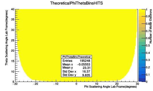
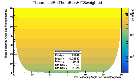
| | + | ===Bin Spacing of 0.05 degrees for θ in Lab Frame=== |
| | + | [[File:TheoryPhiThetaBins05spacing.png]][[File:TheoryPhiThetaBins05spacingWeighted.png]] |
| | | | |
| | + | ===Bin Spacing of 0.1 degrees for θ in Lab Frame=== |
| | + | [[File:TheoryPhiThetaBins1spacing.png]][[File:TheoryPhiThetaBins1spacingWeightedWSigma.png]] |
| | | | |
| − | [[File:TheoreticalWireBinsCorrected.png]][[File:DSigmaVsWireBinCorrected.png]] | + | [[File:CORRELATEDPhiThetaBins1spacing.png]][[File:CORRELATEDPhiThetaBins1spacingWeightedWSigma.png]] |
| | | | |
| − | Using the histogram integral function we find the sum of the values for the wire 1 bin. Collecting the individual <math>d\sigma</math> for each theoretical and physical hits on DC wires.
| + | [[File:ACTUALPhiThetaBins1spacing.png]][[File:ACTUALPhiThetaBins1spacingWeightedWSigma.png]] |
| | | | |
| | + | =Number of Hits on Wires= |
| | + | Not all 1st hits are on layer 1, so we use the correlated theoretical wire number associated with the LUND Theta and Phi values. The theoretical model has events which are detected by physically impossible valued wires. If we limit the lowest wire value to 0.5 and the highest to less than 112.5 |
| | | | |
| | | | |
| − | Wire 1 Based Actual Hits σ=0.00001287 barn
| + | ==Bin Spacing of 0.05 degrees for θ in Lab Frame== |
| | | | |
| − | [[File:Wire1_AcutalHITS.text]]
| + | ==Bin Spacing of 0.1 degrees for θ in Lab Frame== |
| − | [[File:Wire1ActualWeighted.png|left|frame|none|alt=Alt text|σ=0.000013 barn]]
| |
| | | | |
| − | <center><math>\frac{1}{t_{run}}\sum_{\theta_{Lab}}N_{scattered(\theta_{Lab})}=\sum_{\theta(Lab)}\sum_{\phi}\sigma(\theta_{CM})\frac{\sin \theta_{CM}\ \Delta\theta_{CM}\ \Delta\phi_{CM}}{\sin \theta_{Lab}\ \Delta\theta_{Lab}\ \Delta\phi_{Lab}}\Phi \sin \theta_{Lab}\ \Delta\theta_{Lab}\ \Delta\phi_{Lab}</math></center>
| + | [[File:TheoryWireHits1spacing.png]][[File:TheoryWireHits1spacingWeightedwSigma.png]] |
| | | | |
| | | | |
| − | <center><math>\frac{N_{scattered}}{t_{run}}=0.00001287\ \Phi_{nA}</math></center>
| + | [[File:WireBins1stHITSCORRELATED1spacing.png]][[File:WireBins1stHITSCORRELATEDWeightedWSigma1spacing.png]] |
| | | | |
| | + | [[File:WireBins1stHITSACTUAL1spacing.png]][[File:WireBins1stHITSACTUALWeightedWSigma1spacing.png]] |
| | | | |
| − | <center><math>\frac{N_{scattered}}{0.00001287\ \Phi_{nA}}=t_{run}</math></center>
| + | [[File:Sector1HitsMoller1spacing.png]][[File:Sector1HitsMollerWeightedWSigma1spacing.png]] |
| | | | |
| | + | [[File:Sector1HitsNoise1spacing.png]][[File:Sector1HitsNoiseWeightedWSigma1spacing.png]] |
| | | | |
| | + | =Occupancy= |
| | + | LH2_NOSol_0Tor_11GeV_IsotropicPhi_v2_6_ShieldOut |
| | | | |
| − | For 1 hit on wire 1:
| + | Run |
| − | <math>\begin{cases} | + | <pre> |
| − | 3.12\times 10^{11}\ \frac{1}{s}=\Phi_{50nA}\rightarrow t=249ns\\
| + | ./BUILD_GEMC_SIMULATION.sh |
| − | 4.68\times 10^{11}\ \frac{1}{s}=\Phi_{75nA}\rightarrow t=166ns\\
| |
| − | 6.24\times 10^{11}\ \frac{1}{s}=\Phi_{100nA}\rightarrow t=125ns\\
| |
| − | 7.80\times 10^{11}\ \frac{1}{s}=\Phi_{125nA}\rightarrow t=99.6ns\\
| |
| − | 9.36\times 10^{11}\ \frac{1}{s}=\Phi_{150nA}\rightarrow t=83ns
| |
| − | \end{cases}</math>
| |
| | | | |
| | + | </pre> |
| | + | [[ DVMacro ]] |
| | | | |
| | + | ==Clas12Mon== |
| | + | Create hipo file |
| | | | |
| | | | |
| | + | Move hipo file to clas12mon folder |
| | + | <pre> |
| | + | mv LH2_NOSol_0Tor_11GeV_IsotropicPhi_v2_6_ShieldOut.hipo ~/clas12mon |
| | + | </pre> |
| | | | |
| | + | Run monitor program |
| | + | <pre> |
| | + | ./README |
| | + | </pre> |
| | | | |
| | + | Load hipo file |
| | + | <pre> |
| | + | "Press H for hipo" |
| | + | "Press play" |
| | + | "Switch to |
| | + | </pre> |
| | | | |
| | | | |
| | + | ===Clas12mon event counting=== |
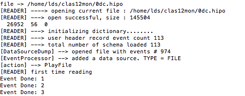
| | + | ====000==== |
| | | | |
| | + | [[File:clas12Count000.png]] |
| | | | |
| − | Wire 1 Based Correlated Hits σ=0.00001345 barn
| + | [[File:000Part1.png]] |
| − | | |
| − | [[File:Wire1_CorrelatedHITS.text]] | |
| − | [[File:Wire1CorrelatedlWeighted.png|left|frame|none|alt=Alt text|σ=0.000013 barn]]
| |
| − | | |
| − | | |
| − | | |
| − | | |
| − | | |
| − | | |
| − | | |
| | | | |
| | + | . |
| | | | |
| | + | . |
| | | | |
| | + | . |
| | | | |
| | + | . |
| | | | |
| | + | [[File:000Part2.png]] |
| | | | |
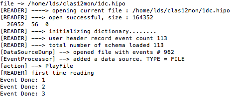
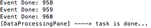
| | + | ====001==== |
| | | | |
| | + | [[File:clas12Count001.png]] |
| | | | |
| | + | [[File:01dchipoPart1.png]] |
| | | | |
| | + | . |
| | | | |
| | + | . |
| | | | |
| | + | . |
| | | | |
| | + | . |
| | | | |
| | + | [[File:01dchipoPart2.png]] |
| | | | |
| | + | ====000 & 001 combined==== |
| | | | |
| | + | [[File:clas12CountCombined000&001.png]] |
| | | | |
| − | Wire 1 Based Theoretical Hits σ=0.00001387 barn
| + | [[File:000&001Part1.png]] |
| | | | |
| − | [[File:Wire1_Based_Angles_and_weight.txt]]
| + | . |
| − | [[File:Wire1TheoreticalWeighted.png|left|frame|none|alt=Alt text|σ=0.000014 barn]]
| |
| | | | |
| − | =Occupancy=
| + | . |
| − | LH2_NOSol_0Tor_11GeV_IsotropicPhi_v2_6_ShieldOut
| |
| | | | |
| − | Run
| + | . |
| − | <pre>
| |
| − | ./BUILD_GEMC_SIMULATION.sh | |
| | | | |
| − | </pre>
| + | . |
| − | [[ DVMacro ]]
| |
| | | | |
| − | ==Clas12Mon==
| + | [[File:000&001Part2.png]] |
| − | Create hipo file
| |
| | | | |
| | | | |
| − | Move hipo file to clas12mon folder
| + | ===evio Counts=== |
| − | <pre>
| |
| − | mv LH2_NOSol_0Tor_11GeV_IsotropicPhi_v2_6_ShieldOut.hipo ~/clas12mon
| |
| − | </pre>
| |
| − | | |
| − | Run monitor program
| |
| − | <pre>
| |
| − | ./README
| |
| − | </pre>
| |
| − | | |
| − | Load hipo file
| |
| − | <pre>
| |
| − | "Press H for hipo"
| |
| − | "Press play"
| |
| − | "Switch to
| |
| − | </pre>
| |
| − | | |
| | | | |
| − | For <math>5^{\circ}>\theta<40^{\circ}\ -30^{\circ}>\phi<30^{\circ}</math>
| + | [[File:evioCountPart1.png]] |
| | | | |
| − | [[File:clas12monNoSolNoShield.png]] | + | [[File:evioCountPart2.png]] |
| | | | |
| | | | |
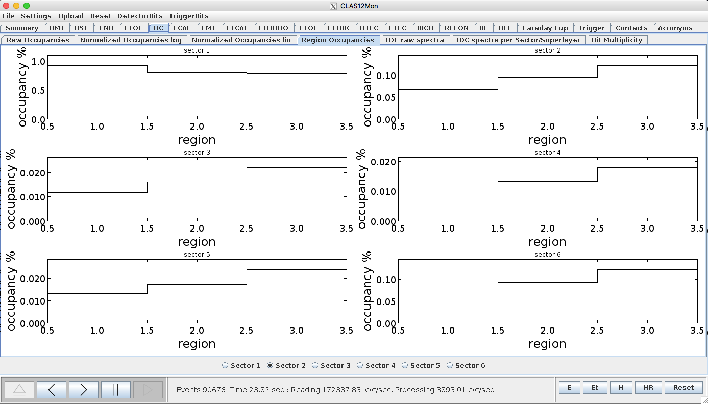
| − | FOR DC Limits | + | ==FOR DC Limits== |
| | | | |
| − | [[File:OccupancyDCLimits_Unweighted.png]] | + | [[File:dcOccupancyUnweighted.png]] |
| | | | |
| | ==Calculating== | | ==Calculating== |
[math]\underline{\textbf{Navigation}}[/math]
[math]\vartriangleleft [/math]
[math]\triangle [/math]
[math]\vartriangleright [/math]
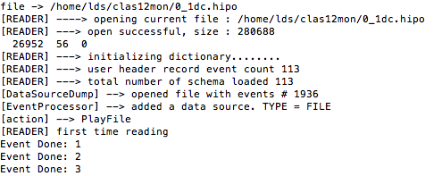
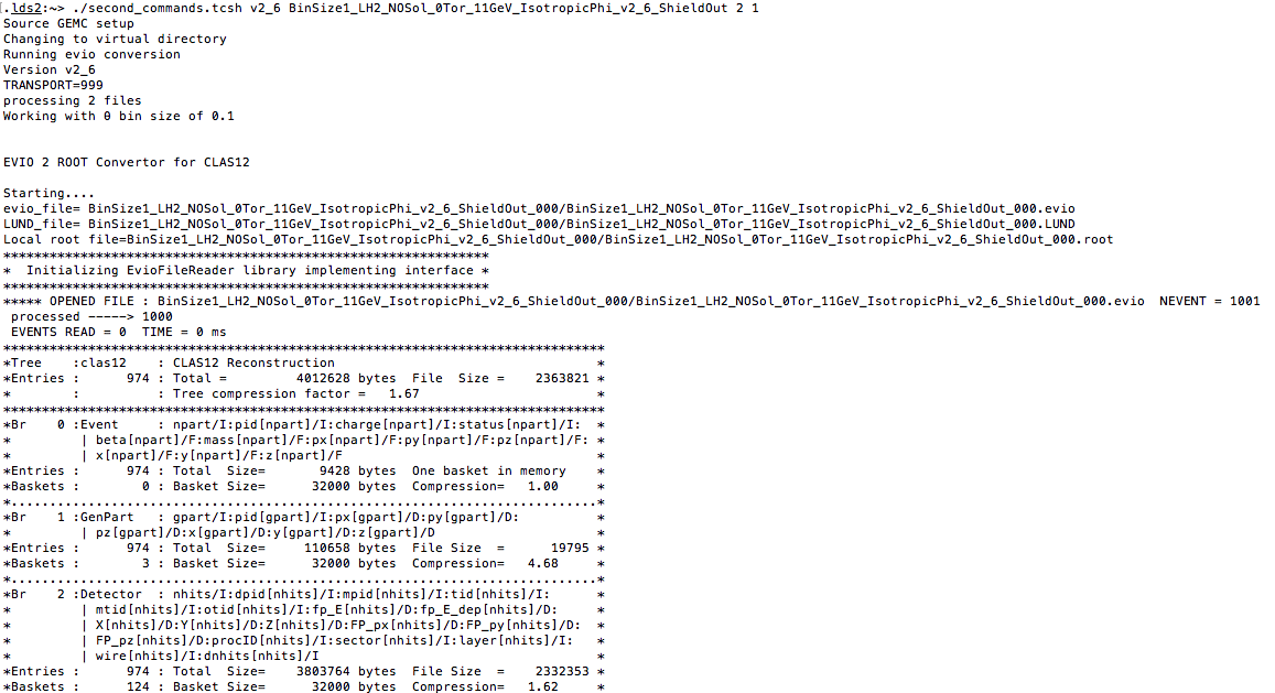
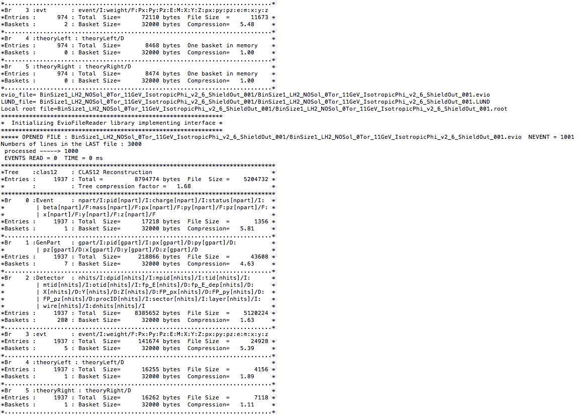
A bash script to run the GEMC simulations is created. tcsh scripts to run root2evio on lds2 is called using sshpass. The lds2 scripts use sshfs
The main script on lds3:
BUILD_GEMC_SIMULATION.sh
The 3 scripts on lds2:
first_commands.tcsh
second_commands.tcsh
last_commands.tcsh
LUND File Output
Uniform spacing in Lab frame, not in CM frame.
0.1 degree spacing for θ in the Lab frame
0.05 degree spacing for θ in the Lab frame
Finding the Cross Section
Total cross section over φ
Total cross section over DC limits
If we make the assumption that the beam of incoming electrons is a flux over an area for a given time,
[math]N_{incident}=\Phi\ A_{beam}\ t_{run} \rightarrow dN_{incident}=\Phi\ dA_{beam}\ t_{run}\rightarrow\ \frac{dN_{incident}}{ dA_{beam}}=\Phi\ t_{run}[/math]
Using the definition of the differential cross section:
[math]\frac{d\sigma}{d\Omega}\equiv \frac{ \Biggl(\frac{dN_{scattered}}{d\Omega} \Biggr)}{\Biggl(\frac{dN_{incident}}{dA}\Biggr)}\rightarrow \frac{d\sigma}{d\Omega}\Biggl(\frac{dN_{incident}}{dA}\Biggr)=\Biggl(\frac{dN_{scattered}}{d\Omega} \Biggr)[/math]
Substituting using the flux
[math] \frac{d\sigma}{d\Omega}\Biggl(\frac{dN_{incident}}{dA}\Biggr)=\Biggl(\frac{dN_{scattered}}{d\Omega} \Biggr)\rightarrow \frac{d\sigma}{d\Omega}\Phi\ t_{run}=\Biggl(\frac{dN_{scattered}}{d\Omega} \Biggr)[/math]
[math]\rightarrow dN_{scattered}= \frac{d\sigma}{d\Omega}\Phi d\Omega= \frac{d\sigma}{d\Omega}\Phi\ t_{run}\ \sin \theta\ d\theta\ d\phi[/math]
Since the differential cross section is known in the Center of Mass frame of reference, but measurements are taken in the Lab Frame, a transformation must occur.
[math]\rightarrow dN_{scattered}= \frac{d\sigma}{d\Omega_{Lab}}\Phi\ t\ \sin \theta_{Lab}\ d\theta_{Lab}\ d\phi_{Lab}[/math]
[math]\frac{d\sigma}{d\Omega_{Lab}}\sin \theta_{Lab}\ d\theta_{Lab}\ d\phi_{Lab}=\frac{d\sigma}{d\Omega_{CM}}\sin \theta_{CM}\ d\theta_{CM}\ d\phi_{CM}[/math]
[math]\frac{d\sigma}{d\Omega_{Lab}}=\frac{d\sigma}{d\Omega_{CM}}\frac{\sin \theta_{CM}\ d\theta_{CM}\ d\phi_{CM}}{\sin \theta_{Lab}\ d\theta_{Lab}\ d\phi_{Lab}}[/math]
[math]\rightarrow dN_{scattered}=\frac{d\sigma}{d\Omega_{CM}}\frac{\sin \theta_{CM}\ d\theta_{CM}\ d\phi_{CM}}{\sin \theta_{Lab}\ d\theta_{Lab}\ d\phi_{Lab}}\Phi\ t_{run}\ \sin \theta_{Lab}\ d\theta_{Lab}\ d\phi_{Lab}[/math]
If we divide both sides by time
[math]\rightarrow \frac{dN_{scattered}}{t_{run}}=\frac{d\sigma}{d\Omega_{CM}}\frac{\sin \theta_{CM}\ d\theta_{CM}\ d\phi_{CM}}{\sin \theta_{Lab}\ d\theta_{Lab}\ d\phi_{Lab}}\Phi \sin \theta_{Lab}\ d\theta_{Lab}\ d\phi_{Lab}[/math]
[math]\rightarrow \frac{dN_{scattered}}{t_{run}}=\frac{d\sigma}{d\Omega_{CM}}\frac{\sin \theta_{CM}\ d\theta_{CM}\ d\phi_{CM}}{\sin \theta_{Lab}\ d\theta_{Lab}\ d\phi_{Lab}}\frac{N_{incident}}{t_{run}} \sin \theta_{Lab}\ d\theta_{Lab}\ d\phi_{Lab}[/math]
[math]\rightarrow \frac{dN_{scattered}}{N_{incident}}=\frac{d\sigma}{d\Omega_{CM}}\sin \theta_{CM}\ d\theta_{CM}\ d\phi_{CM}[/math]
Performing a Riemann sum for [math]-30^{\circ} \lt \phi \lt 30^{\circ}[/math]
The cross section should be equal between both frames since the number of particles is an invariant. The differential cross section must differ between frames since the solid angle does vary.
[math]\sigma_{(CM)}=\sigma{(Lab)}[/math]
[math]\frac{d\sigma}{d\Omega}_{(CM)} d\Omega_{(CM)}=\frac{d\sigma}{d\Omega}_{(Lab)} d\Omega_{(Lab)}[/math]
[math]\frac{d\sigma}{d\Omega}_{(CM)} \sin \theta_{(CM)}\ d\theta_{(CM)}\ d\phi=\frac{d\sigma}{d\Omega}_{(Lab)} \sin \theta_{(Lab)}\ d\theta_{(Lab)}\ d\phi[/math]
From the expression found earlier:
[math]\rightarrow \frac{dN_{scattered}}{N_{incident}}=\frac{d\sigma}{d\Omega_{CM}}\sin \theta_{CM}\ d\theta_{CM}\ d\phi_{CM}[/math]
[math]\rightarrow \frac{d\sigma}{d\Omega}_{(Lab)}=\frac{d\sigma}{d\Omega}_{(CM)} \frac{\sin \theta_{(CM)}\ d\theta_{(CM)}\ d\phi}{ \sin \theta_{(Lab)}\ d\theta_{(Lab)}\ d\phi}[/math]
[math]\rightarrow d\sigma_{(Lab)}=\frac{d\sigma}{d\Omega}_{(CM)} \frac{\sin \theta_{(CM)}\ d\theta_{(CM)}\ d\phi}{ \sin \theta_{(Lab)}\ d\theta_{(Lab)}\ d\phi}\sin \theta_{(Lab)} d\theta_{(Lab)}\ d\phi[/math]
Adjust for DC Sector 1 Limits
GEMC Cross Section
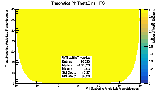
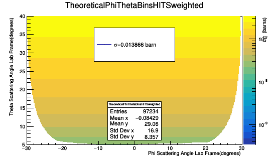
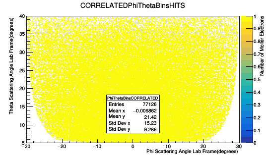
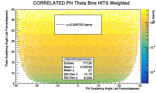
CORRELATED HITS
CORRELATED conditions
| GEMC conditions
|
Meaning
|
| Uses LUND θ and φ values
|
| k=0
|
1st registered hit
|
| dpid[k]=11
|
Electron
|
| tid[k]=2
|
Moller electron from LUND file
|
| mpid[k]=0
|
The mother particle implied from LUND file
|
| sector[k]=1
|
Hit is in sector 1
|
ACTUAL conditions
| GEMC conditions
|
Meaning
|
| Calculates θ and φ values from AVG positions
|
| k=0
|
1st registered hit
|
| dpid[k]=11
|
Electron
|
| tid[k]=2
|
Moller electron from LUND file
|
| mpid[k]=0
|
The mother particle implied from LUND file
|
| sector[k]=1
|
Hit is in sector 1
|
Bin Spacing of 0.05 degrees for θ in Lab Frame
Bin Spacing of 0.1 degrees for θ in Lab Frame
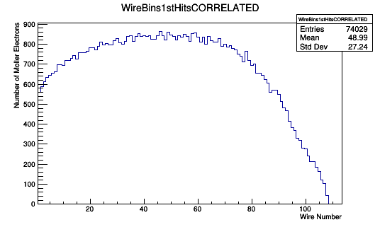
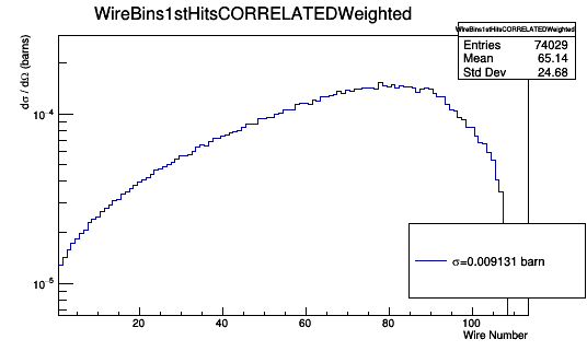
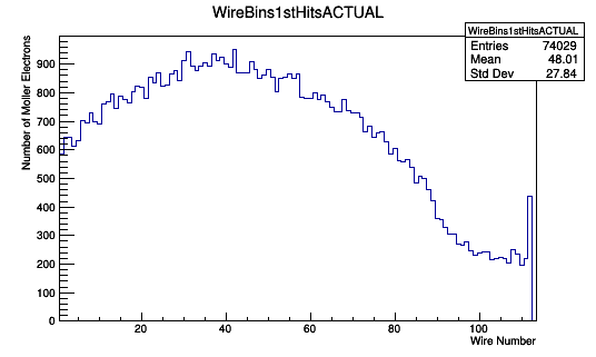
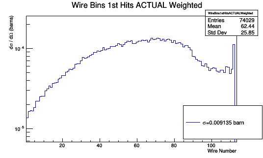
Number of Hits on Wires
Not all 1st hits are on layer 1, so we use the correlated theoretical wire number associated with the LUND Theta and Phi values. The theoretical model has events which are detected by physically impossible valued wires. If we limit the lowest wire value to 0.5 and the highest to less than 112.5
Bin Spacing of 0.05 degrees for θ in Lab Frame
Bin Spacing of 0.1 degrees for θ in Lab Frame
Occupancy
LH2_NOSol_0Tor_11GeV_IsotropicPhi_v2_6_ShieldOut
Run
./BUILD_GEMC_SIMULATION.sh
DVMacro
Clas12Mon
Create hipo file
Move hipo file to clas12mon folder
mv LH2_NOSol_0Tor_11GeV_IsotropicPhi_v2_6_ShieldOut.hipo ~/clas12mon
Run monitor program
./README
Load hipo file
"Press H for hipo"
"Press play"
"Switch to
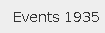
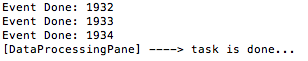
Clas12mon event counting
000

.
.
.
.
001

.
.
.
.
000 & 001 combined
.
.
.
.
evio Counts
FOR DC Limits
Calculating
[math]N_0=\Delta t \cdot R_{events}=\Delta t \cdot \frac{N_{events}}{t_{simulated}}=250\times 10^{-9}\ s \cdot \frac{98181}{9.3\times 10^{-6}\ s}=2639[/math]
[math]Occupancy=\frac{N_{hits}}{N_0}=\frac{N_{hits}}{\Delta t \cdot R_{events}}=\frac{t_{simulated}\cdot N_{hits}}{N_{events}\cdot \Delta t}=[/math]


