LB SageBrushWork PostDefense

Mass Information

The target masses are as follows

50% Se/Sage Sample

Selenium Target (50% Sagebrush Se Mix)	Mass (g)
Outer Front Ni Foil	0.6948
Se Mass	0.51
Outer Se Mass	0.1
Sagebrush Leaves Mass	0.4969

10% Sample

Selenium Target (10% Sagebrush Se Mix)	Mass (g)
Outer Front Ni Foil	0.2783
Se Mass	0.0523
Outer Se Mass	0.0971
Sagebrush Leaves Mass	0.5111

0.1% Se/Sage Sample

Selenium Target (0.1% Sagebrush Se Mix)	Mass (g)
Outer Front Ni Foil	1.1437
Se Mass	0.0559
Outer Se Mass	0.1118
Sagebrush Leaves Mass	50.1080

0.04% Sample

Selenium Target (0.04% Sagebrush Se Mix)	Mass (g)
Outer Front Ni Foil	0.5447
Se Mass	0.0020
Outer Se Mass	0.0992
Sagebrush Leaves Mass	4.9326

Time Cuts

The first step in the PAA process is to identify the time cuts used for the split run. This must be done for all samples (50%,10%,0.1%, and 0.04%).

50% Sage/Se Mixture Time Cuts

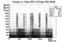
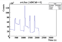
The 50% Se/Sage mixture was measure on Detector B (unshielded, so watch the SNR) on 5/24/17 for a total of 2130.540 seconds. The outer pure witness Se was measure first, and sub-run was roughly 300 seconds for the samples of interest, and 60 seconds for the Co-60 flag. The root command used to draw the timing information was

TTree* tree = MPA;

MPA->Draw("evt.Chan:evt.Sec>>hist2","evt.ADCid == 1");

which produced the histogram below

This seems a little sloppy, lets try a 1D histogram instead to see if the cuts are more clear

ROOT Command: MPA->Draw("evt.Sec>>hist","ADCid==1","");

This produced the histogram below

This seems much cleaner and clearly shows the time cuts

The time cuts are

0-300 (Pure Se)

375-440 (Co-60)

450-700 (Mixture)

715-780 (Co-60)

800-1010 (Pure Se)

1055-1150 (Co-60)

1160-1420 (Mixture)

1425-1495 (Co-60)

1500-1800 (Pure Se)

1810-1870 (Co-60)

1880-2100 (Mixture)

10% Sage/Se Mixture Time Cuts

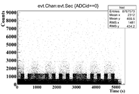
The 10% Se/Sage mixture was measured on Detector A (shielded) on 5/25/17 for a total of 5136.343 seconds. The mixture was measured first, and a sub-run was roughly 300 seconds for the Se samples and 60 seconds for the Co-60 flag. The root commands used were

TTree* tree = MPA;

MPA->Draw("evt.Chan:evt.Sec>>hist2","evt.ADCid == 0");

The time cut information is as follows

0-300 (Mixture)

300-360 (Co-60)

400-640 ( Pure Se)

680-710 (Co-60)

730-1020 (Mixture)

1030-1080 (Co-60)

1100-1360 ( Pure Se)

1400-1440 (Co-60)

1480-1775 (Mixture)

1800-1840 (Co-60)

1875-2150 (Pure Se)

2190-2220 (Co-60)

2250-2550 (Mixture)

2590-2620 (Co-60)

2650-2930 (Pure Se)

2950-3000 (Co-60)

3050-3300 (Mixture)

3390-3350 (Co-60)

3400-3690 (Pure Se)

3700-3750 (Co-60)

3775-4050 (Mixture)

4060-4100 (Co-60)

4120-4400 (Pure Se)

4420-4470 (Co-60)

4480-4770 (Mixture)

4790-4820 (Co-60)

4840-5130 (Pure Se)

0.1% Sage/Se Mixture Time Cuts

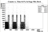
The 0.1% Se/Sage mixture was measured on Detector A (shielded) on 5/24/17 for a total of 2130.540 seconds. The mixture was measured first, and a sub-run was roughly 300 seconds for the Se samples and 60 seconds for the Co-60 flag. The root commands used were

TTree* tree = MPA;

MPA->Draw("evt.Chan:evt.Sec>>hist2","evt.ADCid == 0");

which produced the histogram below

This seems a little sloppy, so let's repeat the procedure for the 50% sample

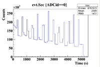
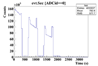
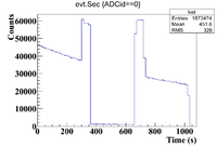
ROOT Command:ROOT Command: MPA->Draw("evt.Sec>>hist","ADCid==0","");

This produced the histogram below

This is again much better than the 2D histogram.

The time cuts are

0-300 (Mixture)

306-340 (Co-60)

376-640 (Pure Se)

650-720 (Co-60)

730-1010 (Mixture)

1020-1050 (Co-60)

1100-1350 (Pure Se)

1400-1460 (Co-60)

1470-1730 (Mixture)

1735-1800 (Co-60)

1804-2140 (Pure Se)

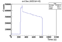
The histogram for the time cuts of the second run is shown below

The time cuts are

0-240 (Outer Se)

245-300 (Co-60)

305-820 (Mixture)

0.04% Sample Time Cuts

The 0.04% Se/Sage mixture was measured on Detector A (shielded) on 5/25/17 for a total of 1711.891 seconds. The mixture was measured first, and a sub-run was roughly 300 seconds for the Se samples and 60 seconds for the Co-60 flag. The root commands used were

TTree* tree = MPA;

MPA->Draw("evt.Sec>>hist2","evt.ADCid == 0");

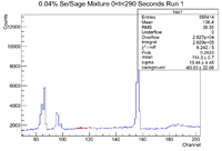
The histogram representing the time cuts for the first run are shown below

The time cuts for this run are

0-290 (Mixture)

295-360 (Co-60)

370-684 (Pure Se)

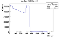
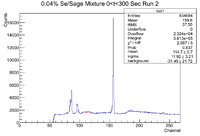
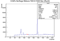
The histogram representing the time cuts for the second run are shown below

The time cuts for this run are

0-300 (Mixture)

305-355 (Co-60)

360-650 (Pure Se)

660-735 (Co-60)

740-1020 (Mixture)

Gamma Spectrum Analysis

50% Sample Analysis

Below is the analysis table for the 50% Se/Sage mixture. The 103 keV line of Se-81m corresponds to a channel # of 130. Due to the sloppiness of the spectrum, I will use a linear + Gaussian fitting function and restrict my analysis to 6 channels because there are other energy lines nearby.

10% Sample Analysis

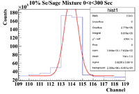
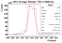
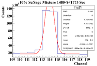
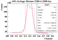
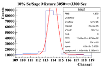
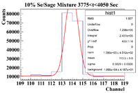
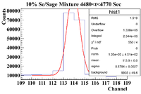
Below is the analysis table for the 10% Se/Sage mixture. The 103 keV line of Se-81m corresponds to a channel # of 113

	0<t<300	730<t<1020	1480<t<1775	2250<t<2550	3050<t<3300	3775<t<4050	4480<t<4770
Thin Window Histogram
Signal in Thin Window	[math] 6.019 \times 10^5 \pm 775.82[/math]	[math] 4.852 \times 10^5 \pm 696.56 [/math]	[math] 4.161 \times 10^5 \pm 645.06 [/math]	[math] 3.667 \times 10^5 \pm 605.56 [/math]	[math] 2.645 \times 10^5 \pm 514.30 [/math]	[math] 2.451 \times 10^5 \pm 495.08 [/math]	[math] 2.344 \times 10^5 \pm 484.15 [/math]
Integrated Background	[math] 2.956 \times 10^5 \pm 885.1 [/math]	[math] 2.074 \times 10^5 \pm 728.7 [/math]	[math] 1.668 \times 10^5 \pm 653.0 [/math]	[math] 1.47 \times 10^5 \pm 606.0 [/math]	[math] 1.115 \times 10^5 \pm 528.6 [/math]	[math] 1.055 \times 10^5 \pm 418.7 [/math]	[math] 9.935 \times 10^4 \pm 496 [/math]
Signal - Background	[math] 3.063 \times 10^5 \pm 1177.01 [/math]	[math] 2.778 \times 10^5 \pm 1008.07 [/math]	[math] 2.493 \times 10^5 \pm 917.88[/math]	[math] 2.197 \times 10^5 \pm 856.70 [/math]	[math] 1.53 \times 10^5 \pm 737.51 [/math]	[math] 1.396 \times 10^5 \pm 648.39 [/math]	[math] 1.35050 \times 10^5 \pm 693.12 [/math]
Runtime (s)	300	290	295	300	250	275	290
Rate (Hz)	[math] 1021 \pm 3.92 [/math]	[math] 957.93 \pm 3.48 [/math]	[math] 845.08 \pm 3.11 [/math]	[math] 732.33 \pm 2.86 [/math]	[math] 612 \pm 2.95 [/math]	[math] 507.64 \pm 2.36 [/math]	[math] 465.69 \pm 2.39 [/math]
Integral Decay Correction (Hz)	[math] 1052.2 \pm 4.04 [/math]	[math] 986.23 \pm 3.58 [/math]	[math] 870.47 \pm 3.20 [/math]	[math] 754.71 \pm 2.95 [/math]	[math] 627.56 \pm 3.03 [/math]	[math] 521.85 \pm 2.43 [/math]	[math] 479.44 \pm 2.46 [/math]
Dead Time (%)	5.06 +/- 0.39	3.06 +/- 0.30	2.53 +/- 0.31	2.26 +/- 0.33	1.92 +/- 0.26	1.65 +/- 0.34	1.55 +/- 0.18
Dead Time Corrected Signal (Hz)
.Dat File Entry For HL Plot

0.1% Sample Analysis

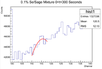
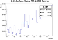
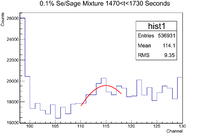
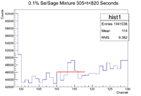
Below is the analysis table for the 0.1% Mixture, the 103 keV line for Se-81m corresponds to a channel # of 113.

	0<t<300	730<t<1010	1470<t<1730	305<t<820 (Run 2)
Thin Window Histogram
Signal in Thin Window	No Signal Visible	No Signal Visible	No Signal Visible	Possible Signal Visible?
Integrated Background	-	-	-	-
Signal - Background	-	-	-	-
Runtime (s)	300	280	260	515
Rate (Hz)	-	-	-	-
Integral Decay Correction (Hz)	-	-	-	-
Dead Time (%)	-	-	-	-
Dead Time Corrected Signal (Hz)	-	-	-	-
.Dat File Entry For HL Plot	-	-	-	-

0.04% Sample Analysis

	0<t<290	0<t<300 (Run 2)	740<t<1020 (Run 2)
Thin Window Histogram
Signal in Thin Window	No Signal Visible	No Signal Visible	No Signal Visible
Integrated Background	-	-	-	-
Signal - Background	-	-	-	-
Runtime (s)	290	300	280
Rate (Hz)	-	-	-	-
Integral Decay Correction (Hz)	-	-	-	-
Dead Time (%)	-	-	-	-
Dead Time Corrected Signal (Hz)	-	-	-	-
.Dat File Entry For HL Plot	-	-	-	-