In the Detector Frame
We can define the constraints of the plane the DC is in
right = ContourPlot[
   x2 == Cot[29.5 \[Degree]] y + .09156, {y, -1, 1}, {x2, 0, 1.8},
   Frame -> {True, True, False, False},
   PlotLabel -> "Right side limit of DC as a function of X and Y",
   FrameLabel -> {"y (meters)", "x (meters)"}, ContourStyle -> Black,
   PlotLegends -> Automatic];

left = ContourPlot[
   x2 == -Cot[29.5 \[Degree]] y + .09156, {y, -1, 1}, {x2, 0, 1.8},
   Frame -> {True, True, False, False},
   PlotLabel -> "Right side limit of DC as a function of X and Y",
   FrameLabel -> {"y (meters)", "x (meters)"}, ContourStyle -> Black,
   PlotLegends -> Automatic];
We can define the x coordinate of the wires as they cross the midpoint plane as shown earlier.
x0forWires[number_] := .23168 + .01337*(number);
We can define the point midway between two parallel lines as the point where one wire is recorded versus its next highest neighbor
x0forWireMiddles[
   number_] := ((.23168 + .01337*(number)) + (.23168 + .01337*(number \
+ 1)))/2;
All of the conditions dependent on and
\[CapitalDelta]a :=
  FullSimplify[(R Sin[\[Theta] \[Degree]])/
     2 (Csc[65 \[Degree] - \[Theta] \[Degree]] -
      Csc[115 \[Degree] - \[Theta] \[Degree]]), \[Theta] > 0];
e := Sin[25 \[Degree]]/Cos[\[Theta] \[Degree]];
a := FullSimplify[(R Sin[\[Theta] \[Degree]])/
     2 (Csc[65 \[Degree] - \[Theta] \[Degree]] +
      Csc[115 \[Degree] - \[Theta] \[Degree]]), \[Theta] > 0];
rD1 := Simplify[(a e - \[CapitalDelta]a) Tan[
     65 \[Degree]] Cos[\[Theta] \[Degree]], \[Theta] > 0];
rD2 := Simplify[(a e + \[CapitalDelta]a) Tan[
     65 \[Degree]] Cos[\[Theta] \[Degree]], \[Theta] > 0];
xD1 := Simplify[rD1 Cos[\[Phi] \[Degree]]];
yD1 := Simplify[rD1 Sin[\[Phi] \[Degree]]];
zD1 := Simplify[rD1 Cot[\[Theta] \[Degree]], \[Theta] > 0];
xD2 := Simplify[rD2 Cos[\[Phi] \[Degree]], \[Theta] > 0];
yD2 := Simplify[rD2 Sin[\[Phi] \[Degree]], \[Theta] > 0];
zD2 := Simplify[rD2 Cot[\[Theta] \[Degree]], \[Theta] > 0];
xP := Simplify[(R Cos[\[Phi] \[Degree]])/(Cot[\[Theta] \[Degree]] +
      Cos[\[Phi] \[Degree]] Cot[65 \[Degree]]), \[Theta] > 0];
yP := Simplify[(R Sin[\[Phi] \[Degree]])/(Cot[\[Theta] \[Degree]] +
      Cos[\[Phi] \[Degree]] Cot[65 \[Degree]]), \[Theta] > 0];
zP := Simplify[(R Cot[\[Theta] \[Degree]])/(Cot[\[Theta] \[Degree]] +
      Cos[\[Phi] \[Degree]] Cot[65 \[Degree]]), \[Theta] > 0];
x1 := Simplify[(rD2^2 - rD1^2 +
       Cot[\[Theta] \[Degree]]^2 (rD2^2 - rD1^2) - 2 xP (xD2 - xD1) -
       2 yP (yD2 - yD1) - 2 zP (zD2 - zD1))/(4 a e) - a e, \[Theta] >
    0];
x := Simplify[x1 - \[CapitalDelta]a + a e, \[Theta] > 0];
xCenter := x + \[CapitalDelta]a;
n := -957.412/(Tan[\[Theta] \[Degree]] + 2.14437) + 430.626;
D2P := Simplify[((xD2 - xP)^2 + (yD2 - yP)^2 + (zD2 -
       zP )^2)^.5, \[Theta] > 0] // N
D1P := Simplify[((xP - xD1)^2 + (yP - yD1)^2 + (zP -
        zD1)^2)^.5, \[Theta] > 0] // N;
y := Simplify[(D1P^2 - x1^2)^.5, \[Theta] > 0] // N;
b := Simplify[a Sqrt[1 - e^2], \[Theta] > 0] // N;
R = 2.52934271645;
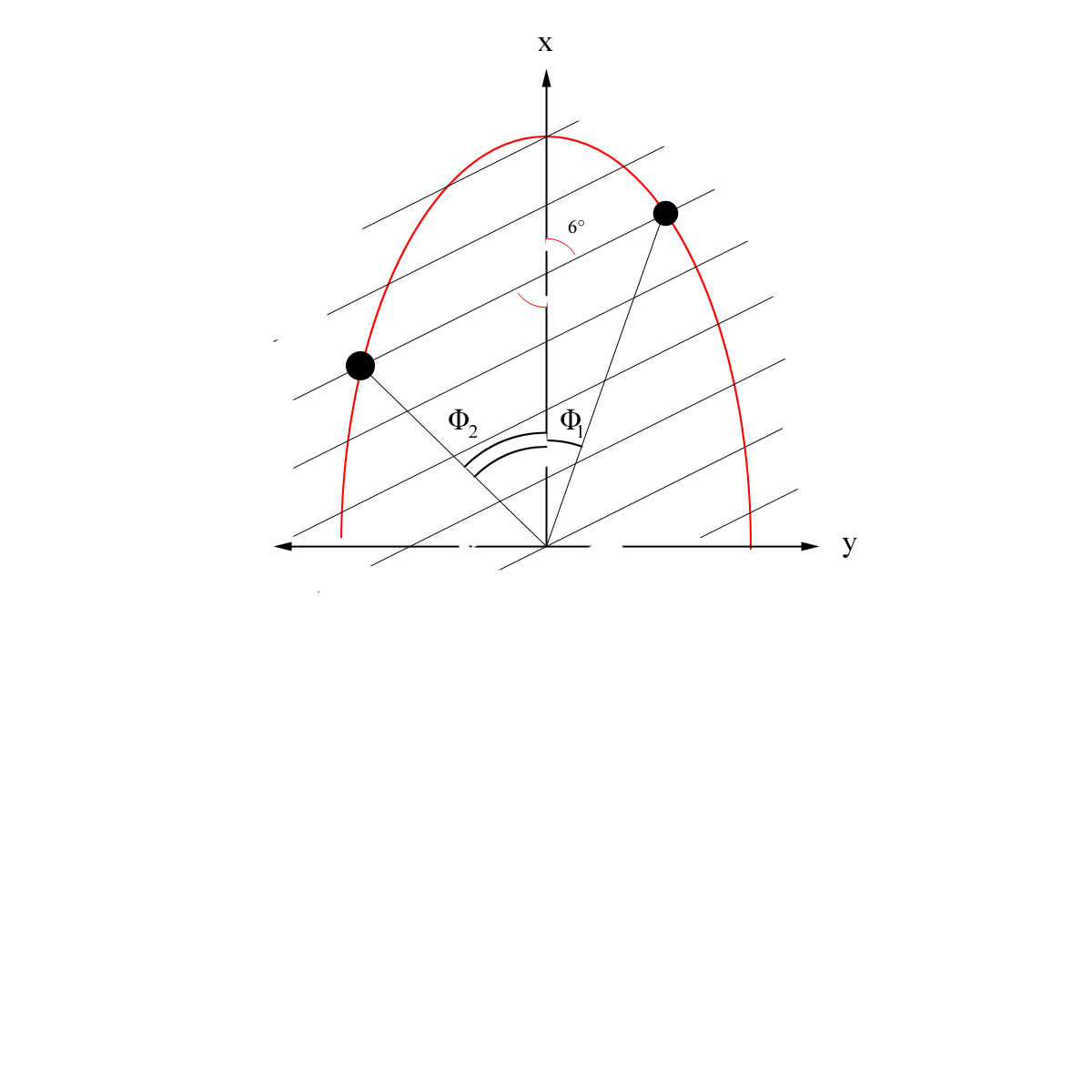
We can define the x-y position on the DC plane as a function of for and limit the angles with the wall on the right and left hand sides. By symmetry these angles are equal, but opposite in sign.
Limits = Table[\[Phi] /.
    NSolve[Sqrt[a^2 (1 - y^2/b^2)] - \[CapitalDelta]a ==
      Cot[29.5 \[Degree]] y + .09156 , \[Phi]], {\[Theta], 5, 40}];
Lim = Table[0, {rows, 1, 36}];
For[rows = 1, rows < 37, rows++,
  For[i = 1, i < 5, i++,
    If[Limits[[rows, i]] > 0 && Limits[[rows, i]] < 40,
      Lim[[rows]] = Limits[[rows, i]];
      ];
    ];
  ];
The angle must have 4 subtracted to equal the line element numbering
In[33]:= Lim[[7 - 4]]

Out[33]= 23.4101
The limit of increases in the plane of the DC sector changes as increases.
In[34]:= Lim[1]

Out[34]= {20.076, 22.024, 23.4101, 24.448, 25.255, 25.9008, 26.4297,
  26.8711, 27.2453, 27.5667, 27.846, 28.0911, 28.3079, 28.5013,
  28.675, 28.8319, 28.9744, 29.1044, 29.2237, 29.3336, 29.4352,
  29.5294, 29.6171, 29.699, 29.7757, 29.8477, 29.9155, 29.9795,
  30.0399, 30.0973, 30.1517, 30.2034, 30.2528, 30.2999, 30.3449,
  30.388}[1]
This limiting condition will record the angle in degrees within an array of wire number(1-112) horizontally and angle vertically
RightSolutions =
  Table[{\[Phi] /.
     Solve[Sqrt[a^2 (1 - y^2/b^2)] - \[CapitalDelta]a ==
       Tan[6 \[Degree]] y +
        x0forWireMiddles[number]  , \[Phi]]}, {\[Theta], 5,
    40}, {number, 1, 112}];
LineRight = Table[{\[Phi], columns}, {rows, 1, 36}, {columns, 1, 112}];
For[rows = 1, rows < 37, rows++,
  For[columns = 1, columns < 113, columns++,
    For[i = 1, i < 5, i++,
      If[RightSolutions[[rows, columns, 1, i]] > 0  &&
         RightSolutions[[rows, columns, 1, i]] < Lim[[rows]],
        LineRight[[rows,
           columns]] = {RightSolutions[[rows, columns, 1, i]],
           columns + .5};
        ];
      ];
    ];
  ];
At =0, the condition of n=-959.637/(tan +2.14437)+430.189 should be met
In[38]:= f[\[Theta]for\[Phi]at0_] := -959.637/(
  Tan[\[Theta]for\[Phi]at0 \[Degree]] + 2.14437) + 430.189

In[39]:= f[40]

Out[39]= 108.538
This implies that for , we know that the wire number to be 108.538. This corresponds to the position being in between 108.5 and 109.5, hence it falls into the 109 "bin".
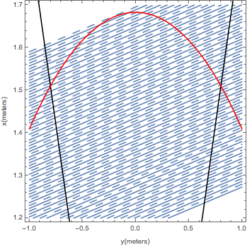
Testing the geometry
ClearAll[\[Theta]];
\[Theta] = 40;
ellipse40 =
  ContourPlot[(x + \[CapitalDelta]a)^2/a^2 + y^2/b^2 == 1, {y, -1,
    1}, {x, 1.2, 1.7}, Frame -> {True, True, False, False},
   PlotLabel ->
    "XY position on DC as a function of \[Phi] for \[Theta]=40\
\[Degree]", FrameLabel -> {"y (meters)", "x (meters)"},
   ContourStyle -> Red, PlotLegends -> Automatic];
Show[Table[
  ContourPlot[
   xWire == Tan[6 \[Degree]] yWire + x0forWires[number], {yWire, -1,
    1}, {xWire, 1.2, 1.7},
   FrameLabel -> {"y(meters)", "x(meters)"}], {number, 70, 109}],
 Table[ContourPlot[
   xWire ==
    Tan[6 \[Degree]] yWire + x0forWireMiddles[number2], {yWire, -1,
    1}, {xWire, 1.2, 1.7},
   ContourStyle -> {Dashing[Large]}], {number2, 70,
   109}], bottom, right, left, ellipse40]
Clearing wire numbers greater than the "wire number" at =0
For[rows = 1, rows < 37, rows++,
  For[columns = 1, columns < 113, columns++,
   If[LineRight[[rows, columns, 2]] > f[rows + 4],
    LineRight[[rows, columns, 1]] = {\[Phi]}
    ]
   ]
  ];
The fact the equation for the y component in the plane of the detector uses a square root function, we know there must be two solutions. Due to the use of inverse trigonometric functions within Mathematica, only the positive values of y will be used. We can find the angle \[Phi] where the elliptical xy path for \[Theta]=40\[Degree] crosses the midway point in between wires. This corresponds to hits at a constant \[Theta] occurring on different wires. The elliptical path hits the right and left wall at \[Phi] = \[PlusMinus]24.9252 and will not cross additional wires lower than this in the 1st quadrant. On the left hand side, the wire number limit is lower since the slope of this plane is positive.
By symmetry, we know that the positions within the 4th quadrant can be reflected into the 1st quadrant by taking the opposite slope of the wire function
ClearAll[\[Theta]];

LeftSolutions =
  Table[{\[Phi] /.
     Solve[Sqrt[
        a^2 (1 - y^2/b^2)] - \[CapitalDelta]a == -Tan[6 \[Degree]] y +
         x0forWireMiddles[number]  , \[Phi]], number}, {\[Theta], 5,
    40}, {number, 1, 112}];
LineLeft =
  Table[{\[Phi], columns}, {rows, 1, 36}, {columns, 1, 112}];
For[rows = 1, rows < 37, rows++,
  For[columns = 1, columns < 113, columns++,
    For[i = 1, i < 7, i++,
     If[LeftSolutions[[rows, columns, 1, i]] > 0  &&
        LeftSolutions[[rows, columns, 1, i]] < Lim[[rows]],
       LineLeft[[rows,
          columns]] = {LeftSolutions[[rows, columns, 1, i]],
          columns + .5};
       ];
     ];
    For[i = 1, i < 6, i++,
     If[LeftSolutions[[rows, columns, 1, i]] > 0  &&
        LeftSolutions[[rows, columns, 1, i]] < Lim[[rows]],
       LineLeft[[rows,
          columns + 1]] = {LeftSolutions[[rows, columns, 1, i]],
          columns + .5};
       ];
     ];
    ];
  ];
We can combine the angles recorded in both quadrants
Collecting the \[Phi] angles as an x variable with the wire as the y variable for a constant value of \[Theta] first for the right hand side
constant\[Theta]right = Table[0, {rows, 1, 36}, {columns, 1, 112}];
constant\[Theta]r = Table[0, {rows, 1, 36}, {columns, 1, 112}];

For[rows = 1, rows < 37, rows++,
 For[columns = 1, columns < 113, columns++,
  constant\[Theta]right[[rows, columns]] = LineRight[[rows, columns]]
  ]
 ]
Flattening the list elements to numerical values
For[rows = 1, rows < 37, rows++,
  constant\[Theta]r[[rows]] =
   Flatten[constant\[Theta]right[[rows]], 2]];
Partitioning the data into {\[Phi],wire number} combinations that increase with respect to the component
For[rows = 1, rows < 37, rows++,
  constant\[Theta]r[[rows]] = Partition[constant\[Theta]r[[rows]], 2]
  ];
Sorting the x values from smallest to largest

