Difference between revisions of "HomeWork Simulations of Particle Interactions with Matter"
| Line 161: | Line 161: | ||
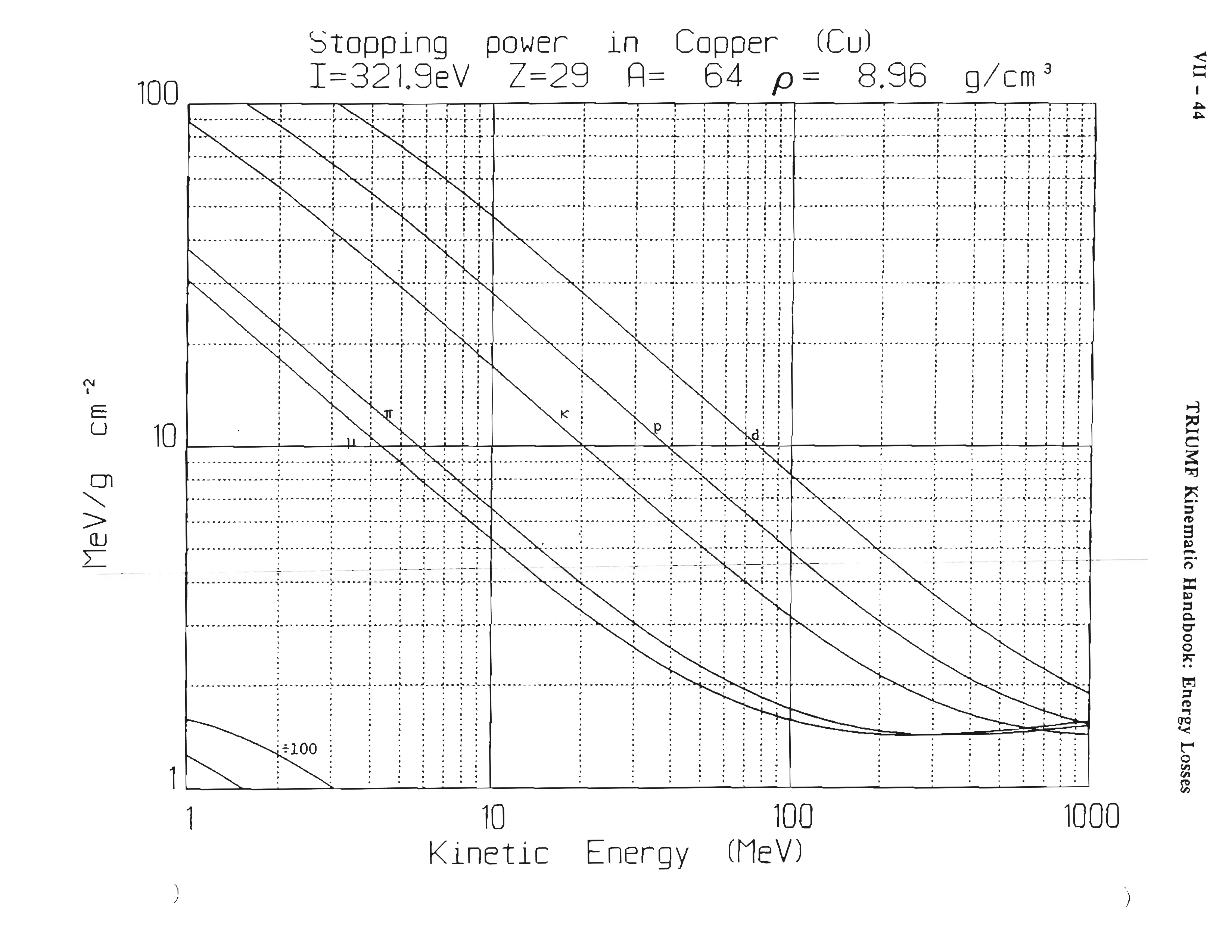
Stopping Power of several particles through Copper as a function of energy is shown in this curve. [[Image:StoppingPowerInCopper.pdf]] | Stopping Power of several particles through Copper as a function of energy is shown in this curve. [[Image:StoppingPowerInCopper.pdf]] | ||
| − | [[ | + | [[File:StoppingPowerInCopper.png]] |
| − | [[Image:HiResStoppingPowerInCopper.png]] | + | [[Image:HiResStoppingPowerInCopper.png | 200 px]] |
[http://www.datathief.org/ Data Thief] | [http://www.datathief.org/ Data Thief] | ||
Revision as of 16:10, 30 September 2016
Homework 1
Apply for an account on minerve
request an account on the minerve cluser using the link below
http://help.cose.isu.edu/services/compute-clusters/request-cluster-access
1.) Maxwell Boltzmann
Given the Maxwell -Boltzmann Distribution
a.) Show <v>
Show that
b.) Energy Fluctuation (Grad)
Show that the energy fluctuation is
- Note
- = velocity fluctuation
2.) MC calculation of Pi
Calculate using the Monte Carlo method described in the Notes
You may use the program I gave you in the lab for this but you must change the program to indicate that you were able to understand its structure and you were able to recompile it.
Xtra help: http://physics.isu.edu/~tforest/Classes/NucSim/Day1/PI_MC/
3.) Histograms using ROOT
Create histograms of the random numbers stored a the ROOT ntuple .
First step is to create a file with the 2 columns of random numbers in it.
./PI_MC 1000 > temp.dat
now load the program "ascii2root.C" into ROOT.
Add the program ROOT to your UNIX path with the command below
source ~foretony/src/ROOT/root-6.06.02/bin/thisroot.sh
Now run the root program
root -l
now load the asci2root program into ROOT
root [0] .L ascii2root.C
now run the program so it reads the data in from the file "temp.dat" created above
root [1] asci2nt("temp.dat")
You now have a ROOT file called "rns.root"
for simplicity lets quite root and restart it
root [2] .q
now restart it and tell it to load the root file "rns.root" .
root -l rns.root
You don't have to do it this way. You could use the browser to load it "new TBrowser()".
root [1] new TBrowser();
Look under the "ROOT Files" menu and you will see and icon labeled "rns.root".
Double click on the icon labeled "rns.root"
You now see a folder icon named "rns"
Double click again.
You now see a leaf icon with the names "rnd1" and "rnd2". These should contain the numbers from the file temp.dat.
double click on one of the leaf icons and a histogram will appear.
now try some of the commands below.
rns->Draw("rnd1*4");
rns->Draw("rnd1:rnd1","rnd1>0.5");
rns->Draw("asin(rnd1)");
rns->Draw("asin(rnd1-rnd2)");   Does this look like a Normal/Gaussian Distributi
on?
Some reference material:
http://physics.isu.edu/~tforest/Classes/NucSim/Day1/RNG/Marsaglia/noviceExample/
Homework 2
1.) Derive Rutherford Formula
Derive the Rutherford Scattering formula following the approach used in the notes for the elastic scattering of two impenetrable spheres of diameter . TF_SPIM_Intro#Example_4:_Elastic_Scattering
2.) Compile and Install your own version of GEANT4
see
or step by step instructions at
At this time GEANT4 versions newer than 4.9.6 will not install on minerve because of minerve's old operating system.
2.) EXN02 in GEANT
You will learn how to setup your Unix environment to compile EXN02 from the GEANT4 distribution
a.) Compile and run the default version of ExN02 in GEANT4
You can use a computer screen shot to prove you did this.
b.) Now make your own copy of it and change the target material
Homework 3
1.) Use GEANT4 to simulate the calculation of energy loss for a charged particle traversing LH2. In class I showed an example for an incident 10 MeV proton. You need to pick another particle (pion, kaon, muon ...) and a different energy. Compare your answer with the Triumf curveFile:SPIM HydrogenStoppingPower.pdf.
2.) Compute for the heavy charged particle you chose to simulate in problem 1. Use the particle's energy at one of the tracking steps and compare to what GEANT4 found.
3.) Graph dE/dX -vs- E for E between 1 and 10 MeV.
Homework 4
1.) Show that the maximum energy transfered to thin absorbers for a relativistic head on collision is
- = momentum of incident heavy charged ion of mass
- = mass of target electron initially at rest
2.) Use GEANT4 to determine the Range of the particle chosen in Homework 3 through liquid hydrogen as a function of at least three of the Energies used in Homework 3.
Homework 5
1.) You need to lower the beam energy of 600 MeV protons to 400 MeV using a slab of copper. The density of the copper is 8.962 . Determine how thick the copper should be by integrating the stopping power curve:
Stopping Power of several particles through Copper as a function of energy is shown in this curve. File:StoppingPowerInCopper.pdf


2.) Alter GEANT4 example N02 to check your answer for problem 1 above. I expect you to hand in a screen shot showing GEANT4 tracking the proton from 600 MeV to 400 MeV.
3.) Find using GEANT4 for a 600 MeV proton traveling through a slab of copper. You will need to make the copper thick enough to stop the proton. Then output the stopping distance to a file which you can read into ROOT using some of the software we used for Homework 1's RNG problem.
Homework 6
Media:SPIM_BremE-Spectrum-Tantalum.pdf
Media:SPIM_LaTex_TemplateFile.txt
File:SPIM LaTex TemplateFile.txt
Homework 7
Homework 8
Homework 9
1.) Write a Paragraph (4 - 5 sentences) describing the Simulation you would like to perform as your Project for this class. You will need to write a title. You will need to specify the reaction you will be simulating.
Use the Latex skeleton file below to format your document
Media:SPIM_LaTex1_TemplateFile.txt
some commands:
latex filename
dvips filename -o temp.ps
pdflatex filename
Homework 10
There are 2 parts to this homework. First you will compare relative rates for the PhotoElectric, Compton, and pair production physics processes using the same target you used in Homework 10. Second you will write another section of your project which describes the experimental results you are going to compare to using GEANT4.
1.) Compare Photoelectric, Compton and pair production rates relative to eachother using the same target used in the last Homework assignment (#10).
a.) first turn on all three physics processes for a gamma particle in the physics list.
b.) add variables to the output which can be used to identify which physics process is responsible for the event being written to the output file.
c.) Run the simulation so the incident photon energy spans energies from 100 eV to 10 GeV.
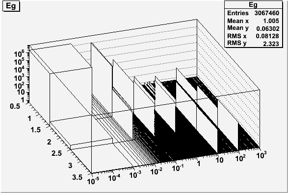
d.) Use ROOT to plot a 3-D representation of the Process type on one axis, the incident photon energy on the other axis and the number of counts along the z-axis.
A bad example of such a plot for a 30 cm long Argon gas target is given in the file
Yours will have better labels
Hint:
->Draw("ProcesID:Egamma","","lego");
->Draw("evt.ProcessID:evt.Ebeam >> (20000,0,200,3,0.5,3.5)","","lego");
2.) Add another section to your project report which describes the experimental measurements you will be using to compare to GEANT4. I am expecting to see a plot and references.
Homework 11
The objective of this homework is to compare the number of collisions needed to thermalize a neutron in GEANT to the expected number of collisions using the Neutron Slowing Down Theory described in class.
1.) Add neutron physics process to your physics list
#include "G4HadronElasticProcess.hh"
#include "G4NeutronHPElasticData.hh"
#include "G4NeutronHPElastic.hh"
#include "G4NeutronHPThermalScatteringData.hh"
#include "G4NeutronHPorLElastic.hh"
   } else if (particleName == "neutron") {
     //neutron
     //G4NeutronHPElastic* elasticModel = new G4NeutronHPElastic();
     G4NeutronHPorLElastic* elasticModel = new G4NeutronHPorLElastic();
    // define process to handle elastic scattering
     G4HadronElasticProcess* hadElastProc = new G4HadronElasticProcess();
    // register the model you are using for eleastic scattering
     hadElastProc->RegisterMe(elasticModel);
   // add the elastic scattering process to the process manager
     G4ProcessManager* pmanager = G4Neutron::Neutron()-> GetProcessManager();
     pmanager->AddDiscreteProcess(hadElastProc);
}
Use a Liquid Hydrogen target
 G4Material* LH2 =
   new G4Material("Hydrogen", z=1., a= 1.01*g/mole, density= 0.07*g/cm3, kStateGas,3*kelvin,1.7e5*pascal);
change the target to be a 60 cm square and 60 cm thick in Z (a 60 cm cube)
fTargetLength = 60 * cm; // Full length of Target
solidTarget = new G4Box("target",fTargetLength,fTargetLength,targetSize);
Simulations_of_Particle_Interactions_with_Matter Back to Notes
