Forest UCM RBM

Rigid Body Motion

Rigid Body

Rigidy Body

A Rigid Body is a system involving a large number of point masses, called particles, whose distances between pairs of point particles remains constant even when the body is in motion or being acted upon by external force.

Forces of Constraint

The internal forces that maintain the constant distances between the different pairs of point masses.

Total Angular Momentum of a Rigid Body

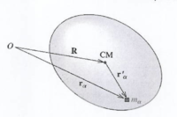
Consider a rigid body that rotates about a fixed z-axis with the origin at point O.

let

[math]\vec R[/math] point to the center of mass of the object

[math]\vec {r}_k[/math] points to a mass element [math]m_k[/math]

[math]\vec{r}_k^{\;\;\prime}[/math] points from the center of mass to the mass element [math]m_k[/math]

the angular momentum of mass element [math]m_k[/math] about the point O is given as

[math]\ell_k = \vec {r}_k \times \vec {p}_k = \vec {r}_k \times m \vec {\dot r}_k[/math]

The total angular momentum about the point O is given as

[math] \vec L = \sum \ell_k = \sum \vec {r}_k \times m_k \vec {\dot r}_k[/math]

This can be cast in term of the angular momentum about the center of mass and the angular momentum of the CM motion

[math]\vec {r}_k = \vec R + \vec{r}_k^{\;\; \prime}[/math]

[math] \vec L = \sum \vec {r}_k \times m_k \vec {\dot r}_k[/math]

[math] = \sum (\vec R + \vec{r}_k^{\;\; \prime}) \times m_k (\vec \dot R + \vec{\dot r}_k^{\;\; \prime})[/math]

[math] = \sum \vec R \times m_k \vec \dot R + \sum \vec R \times m_k \vec{\dot r}_k^{\;\; \prime} + \sum \vec{r}_k^{\;\; \prime} \times m_k \vec \dot R +\sum \vec{r}_k^{\;\; \prime} \times m_k \vec{\dot r}_k^{\;\; \prime} [/math]

[math]\sum \vec R \times m_k \vec \dot R = \vec R \times \sum m_k \vec \dot R = \vec R \times M \vec \dot R = \vec R \times \vec P[/math]

[math]\vec P =[/math] momentum of the center of Mass

[math]\sum \vec R \times m_k \vec{\dot r}_k^{\;\; \prime} = \vec R \times \sum m_k \vec{\dot r}_k^{\;\; \prime} [/math]

[math]\sum m_k \vec{\dot r}_k^{\;\; \prime} = \sum m_k \left ( \vec {r}_k - \vec R\right ) = \sum m_k \vec {r}_k - \sum m_k \vec R = \vec {v}_{cm} - \vec{v}_{cm} = 0[/math]

The location of the center of mass is at [math]\vec{ r}_k^{\;\; \prime} = 0[/math] the derivative is also zero

[math]\sum \vec{r}_k^{\;\; \prime} \times m_k \vec \dot R = \sum m_k \vec{r}_k^{\;\; \prime} \times \vec \dot R =0 [/math] : The location of the CM is at 0

[math] \vec L = \vec R \times \vec P + \sum \vec{r}_k^{\;\; \prime} \times m_k \vec{\dot r}_k^{\;\; \prime} [/math]

[math] = L_{\mbox{CM}} + L_{\mbox{about CM}} [/math]

The total angular momentum is the sum of the angular momentum of the center of mass of a rigid body [math] L_{\mbox{CM}} [/math] and the angular momentum of the rigid body about the center of mass [math] L_{\mbox{about CM}} [/math]

Planet example

What is the total angular momentum of the earth orbiting the sun?

There are two components

[math] \vec L_{\mbox{CM}} [/math] = angular momentum of the earth orbiting about the sun

[math] \vec L_{\mbox{about CM}} [/math] = angular momentum of the earth orbiting about the earth's center of mass (Spin)

[math]\vec L_{\mbox{tot}} = \vec L_{\mbox{CM}} + \vec L_{\mbox{about CM}}[/math]

[math] \vec L_{\mbox{CM}} [/math] is conserved and defined as Orbital angular momentum

[math]\vec \dot L_{\mbox{CM}} = \vec \dot R \times \vec P + \vec R \times \vec \dot P[/math]

[math]\vec \dot R \times \vec P = \vec V \times M \vec V = 0[/math]

[math]\Rightarrow \vec \dot L_{\mbox{orb}} = \vec R \times \vec \dot P=\vec R \times \vec {F}_{ext}[/math]

If there is only a central force

[math]\vec {F}(\mbox{ext}) = G \frac{Mm}{R^3} \vec R[/math]

Then

[math]\vec R \times \vec {F}(\mbox{ext}) = \vec R \times G \frac{Mm}{R^3} \vec R= G \frac{Mm}{R^3} \vec R \times \vec R =0 [/math]

Thus

[math]\vec \dot L_{\mbox{CM}} = \vec R \times \vec {F}(\mbox{ext}) = 0[/math]

[math]\vec L_{\mbox{CM}} \equiv \vec L_{\mbox{Orb}}[/math] = constant = Orbital angular momentum

The above is a good approximation even though the Sun's gravitational Field is not perfectly uniform

How about [math]\vec L_{\mbox{about CM}}[/math]?

Since

[math]\vec L_{\mbox{tot}} = \sum \vec {r}_k \times m_k \vec {\dot r}_k =\vec L_{\mbox{Orb}} + \vec L_{\mbox{about CM}}[/math]

as seen earlier

[math] \vec L = \sum \vec {r}_k \times m_k \vec {\dot r}_k[/math]

[math] = \sum (\vec R + \vec{r}_k^{\;\; \prime}) \times m_k (\vec \dot R + \vec{\dot r}_k^{\;\; \prime})[/math]

[math] = \vec R \times \vec P + \sum \vec{r}_k^{\;\; \prime} \times m_k \vec{\dot r}_k^{\;\; \prime} [/math]

Then

[math]\dot \vec L = \vec \dot R \times \vec P +\vec R \times \vec \dot P + \sum \vec{\dot r}_k^{\;\; \prime} \times m_k \vec{\dot r}_k^{\;\; \prime} + \sum \vec{r}_k^{\;\; \prime} \times m_k \vec{\ddot r}_k^{\;\; \prime} [/math]

[math] =\vec R \times \vec \dot P + \sum \vec{r}_k^{\;\; \prime} \times m_k \vec{\ddot r}_k^{\;\; \prime} [/math]

[math] =\vec R \times \vec {F}(\mbox{ext}) + \sum \vec{r}_k^{\;\; \prime} \times m_k \vec{\ddot r}_k^{\;\; \prime} [/math]

[math] =\vec{\dot{ L}}_{\mbox{Orv}} + \vec{\dot {L}}_{\mbox{about CM}}[/math]

[math]\Rightarrow \vec{\dot {L}}_{\mbox{about CM}} = \sum \vec{r}_k^{\;\; \prime} \times m_k \vec{\ddot r}_k^{\;\; \prime} [/math]

[math] \vec{\dot {L}}_{\mbox{spin}}\equiv\vec{\dot {L}}_{\mbox{about CM}} = \sum \vec{r}_k^{\;\; \prime} \times m_k \vec{\ddot r}_k^{\;\; \prime} \equiv \tau(\mbox{ext about CM}) [/math]

The total angular momentum is the sum of the orbital angular momentum and the spin

[math]\vec L_{\mbox{tot}} = \vec L_{\mbox{orb}} + \vec L_{\mbox{spin}}[/math]

Precession of the Earth

http://courses.physics.northwestern.edu/Phyx125/Precession%20of%20the%20Earth.pdf

Total Kinetic energy of a Rigid Body

Using the same coordinate system as above

the kinetic energy of mass element [math]m_k[/math] about the point O is given as

[math]T_k = \frac{1}{2} m_k \left | \vec \dot{r}_k \right |^2[/math]

The total Kinetic about the point O is given as

[math] \vec T = \sum \frac{1}{2} m_k \left | \vec \dot{r}_k \right |^2[/math]

Rewriting this again in terms of the location of the CM of the body [math]\vec R[/math] and the location of a mass element from the CM [math]\vec{r}_k^{\;\; \prime}[/math]

[math]\vec {r}_k = \vec R + \vec{r}_k^{\;\; \prime}[/math]

[math]\vec {\dot r}_k = \vec \dot R + \vec{\dot r}_k^{\;\; \prime}[/math]

[math]\vec {\dot r}_k \cdot \vec {\dot r}_k = \left ( \vec \dot R + \vec{\dot r}_k^{\;\; \prime} \right ) \cdot \left ( \vec \dot R + \vec{\dot r}_k^{\;\; \prime} \right ) [/math]

[math] = \left | \vec \dot R \right |^2 + \left | \vec{\dot r}_k^{\;\; \prime} \right |^2 + 2 \vec \dot R \cdot \vec{\dot r}_k^{\;\; \prime} [/math]

[math] \vec T = \sum \frac{1}{2} m_k \left | \vec \dot{r}_k \right |^2[/math]

[math] = \sum \frac{1}{2} m_k \left | \vec \dot R \right |^2 + \left | \vec{\dot r}_k^{\;\; \prime} \right |^2 + 2 \vec \dot R \cdot \vec{\dot r}_k^{\;\; \prime}[/math]

[math] = \frac{1}{2} M \left | \vec \dot R \right |^2 + \frac{1}{2} \sum m_k \left | \vec{\dot r}_k^{\;\; \prime} \right |^2 + \vec \dot R \cdot \sum m_k \vec{\dot r}_k^{\;\; \prime}[/math]

For a Rigid body

[math] \sum m_k \vec{\dot r}_k^{\;\; \prime} =0 [/math] The internal kinetic energy is zero for a rigid body, otherwise it would be expanding

[math] \vec T = \frac{1}{2} M \left | \vec \dot R \right |^2 + \frac{1}{2} \sum m_k \left | \vec{\dot r}_k^{\;\; \prime} \right |^2 \cdot [/math]

[math] = T_{\mbox{CM}} + T_{\mbox{about CM}}[/math]

Total Potential energy of a Rigid Body

If all forces are conservative

[math]\vec \nabla \times \vec F_{ij} = 0[/math]

then a Potential Energy may be defined

[math]\Delta U_{ij}(r_{ij}) \equiv -\int_{r_o}^r \vec{F}_{ij}(r_{ij}) \cdot d\vec{r}_{ij} = - W_{cons}[/math]

Then the potential energy of a rigid body is given by

[math]\sum_{i\lt j} \Delta U_{ij}(r_{ij}) = U_{\mbox{int}} = [/math] constant

for a rigid body the inter-particle separation distance [math]r_{ij}[/math] is constant so the internal potential of a rigid body does not change

Thus the kinematics of a Rigid body only needs to consider the potential energy of external forces.

Rotation about a fixed axis

Consider a Rigid body rotating with a speed [math]\vec \omega[/math] about a fixed axis (z-axis) with its origin at the point O

[math]\vec \omega = \omega \hat k[/math]

The total angular momentum about the point O is given as

[math] \vec L = \sum \ell_k = \sum \vec {r}_k \times m_k \vec {\dot r}_k[/math]

As seen in the non-inertial reference frame chapter

[math]\vec \dot r = \vec v = \vec \omega \times \vec r[/math]

thus

[math] \vec \omega \times \vec r_k = \left( \begin{array}{ccc} \hat i & \hat j & \hat k\\ 0 & 0 & \omega \\x_{k} & y_{k} & z_{k}\end{array} \right)= \omega \left ( - y_{k} \hat i + x_{k} \hat j \right ) [/math]

[math] \vec {r}_k \times \vec {\dot r}_k = \vec {r}_k \times \vec \omega \times \vec r = \vec {r}_k \times \omega \left ( - y_{k} \hat i + x_{k} \hat j \right ) [/math]

[math]= \left( \begin{array}{ccc} \hat i & \hat j & \hat k\\ x_{k} & y_{k} & z_{k} \\ -\omega y_{k} & \omega x_{k} & 0\end{array} \right)= \omega \left ( - z_{k}x_{k} \hat i - z_{k}y_{k} \hat j + \left (x_{k}^2+y_{k}^2 \right ) \hat k \right ) [/math]

[math] \vec L = \sum \ell_k = \sum \vec {r}_k \times m_k \vec {\dot r}_k[/math]

[math] = \omega \sum m_k \left ( - z_{k}x_{k} \hat i - z_{k}y_{k} \hat j + \left (x_{k}^2+y_{k}^2 \right ) \hat k \right )[/math]

Moments (Products) of Inertia about the fixed axis

As seen above, the angular momentum of a rigid body rotating about a fixed axis ( the z-axis in this case) is given by

[math] \vec L = \sum \ell_k = \sum \vec {r}_k \times m_k \vec {\dot r}_k[/math]

[math] = \omega \sum m_k \left ( - z_{k}x_{k} \hat i - z_{k}y_{k} \hat j + \left (x_{k}^2+y_{k}^2 \right ) \hat k \right )[/math]

Although the object was only rotating about the z-axis, there can be angular momentum components along the other directions

In other words, unlike what you learned in introductory physics

[math]\vec L \ne I \vec \omega[/math] in general

instead the general expression for angular momentum is

[math]\vec L = \vec r \times \vec p[/math] is the more general statement

The Moment of Inertia is the inertia of the rotating body for the angular momentum that is parallel to the angular velocity The other components of the angular momentum that are not along the direction of the angular velocity related to the angular velocity by the Product of Inertia

The Moment of Inertia for the above example is defined as

[math]L_z = \omega \sum m_k \left (x_{k}^2+y_{k}^2 \right )[/math]

Let

[math]I_{zz} \equiv \sum m_k \left (x_{k}^2+y_{k}^2 \right ) =[/math] moment of inertia about the z-axis in the "z" ([math]\hat k[/math]) direction.

Then

[math]L_z = I_{zz} \omega[/math]

Similarly

The product of Inertia of a rigid body rotating about the z-axis for the angular momentum component along the x-axis is given by

[math]I_{xz} \equiv \sum m_k(-x_{k} z_{k}) [/math]

The product of Inertia of a rigid body rotating about the z-axis for the angular momentum component along the y-axis

[math]I_{yz} \equiv \sum m_k \left (-y_{k} z_{k} )\right ) [/math]

Note the negative sign is indicative of the rigid body's resistance (inertia) to have an angular momentum component that is not in the same direction as its rotation.

[math] \vec L =\omega \left ( I_{xz} \hat i + I_{yz} \hat k + I_{zz} \hat k \right )[/math] = angular momentum about the z-axis

Example

Moment of Inertia of a sphere

Find the moment of inertia of a uniform solid sphere of Radius (R) and mass (M) about its diameter.

Using a coordinate system with its origin at the center of the sphere

For a set of discrete masses

[math]I_{zz} \equiv \sum m_k \left (x_{k}^2+y_{k}^2 \right ) =[/math] moment of inertia about the z-axis in the "z" ([math]\hat k[/math]) direction.

For a mass distribution the above summation is written in integral form as

[math]I_{zz} = \int dm_k \left (x_{k}^2+y_{k}^2 \right ) [/math]

one may define the sphere's density as

[math]\rho = \frac{M}{\frac{4}{3} \pi R^3}[/math]

A differential mass is written as

[math]dm_k = \rho dV_k = [/math] Imagine a differential circle in the x-y plane that you integrate along z

if using spherical coordinates

[math]x_k = r \sin \theta \cos \phi \;\;\;\; y_k = r \sin \theta \sin \phi[/math]

[math]x_k^2 + y_k^2 = r^2 \sin^2 \theta[/math]

[math]I_{zz} = \int dm_k \left (x_{k}^2+y_{k}^2 \right ) [/math]

[math]= \rho \int r^2 dV_k = \rho \int (r \sin \theta )^2 dV_k = \rho \int r^2 \sin^2 \theta (r^2 dr \sin \theta d \theta d \phi)[/math]

[math]= \rho \int_0^R r^4 dr \int_0^{\pi} \sin^3 \theta d \theta \int_0^{2\pi} d \phi[/math]

[math]= \frac{8 \pi}{15} \rho R^5 = \frac{2}{5} MR^2[/math]

[math]dV = r^2 dr \sin \theta d \theta d \phi[/math]

The moment of Inertia of a hollow sphere of outer radius [math]b[/math] and inner radius [math]a[/math]

Moments of Inertia, like masses, add and subtract like scalers.

[math]I(b,a) = I(b,0) - I(a,o) = \frac{8 \pi}{15} \rho (b^5 - a^5)[/math] = Moment of inertia of a sphere of inner radius [math]a[/math] and outer radius [math]b[/math].

[math]\rho = \frac{M}{V} = \frac{M}{\frac{4 \pi}{3} (b^3 - a^3)}[/math]

[math]I(b,a) = \frac{2}{5} M \frac{ (b^5 - a^5)}{ (b^3 - a^3)}[/math] = Moment of inertia of a sphere of inner radius [math]a[/math] and outer radius [math]b[/math].

Moment of inertia tensor

The angular momentum for a body spinning about an arbitrary axis.

let

[math]\vec \omega = \omega_x \hat i + \omega_y \hat j + \omega_z \hat k[/math]

Consider a Rigid body rotating with a speed [math]\vec \omega[/math] about a fixed axis (z-axis) with its origin at the point O

[math]\vec \omega = \omega \hat k[/math]

The total angular momentum about the point O is given as

[math] \vec L = \sum \ell_k = \sum \vec {r}_k \times m_k \vec {\dot r}_k= \sum m_k \left [ \vec {r}_k \times \vec {\dot r}_k \right ][/math]

As seen in the non-inertial reference frame chapter

[math]\vec \dot r = \vec v = \vec \omega \times \vec r[/math]

thus

[math] \vec \omega \times \vec r_k = \left( \begin{array}{ccc} \hat i & \hat j & \hat k\\ \omega_x & \omega_y & \omega_z \\x_{k} & y_{k} & z_{k}\end{array} \right)= \left ( \omega_y z_{k} - \omega_z y_k \right ) \hat i + \left ( \omega_z x_{k} - \omega_x z_k \right ) \hat j + \left ( \omega_x y_{k} - \omega_y x_k \right ) \hat k [/math]

[math] \vec {r}_k \times \vec {\dot r}_k = \vec {r}_k \times \vec \omega \times \vec r = \vec {r}_k \times \omega \left ( - y_{k} \hat i + x_{k} \hat j \right ) [/math]

[math]= \left( \begin{array}{ccc} \hat i & \hat j & \hat k\\ x_{k} & y_{k} & z_{k} \\ \left ( \omega_y z_{k} - \omega_z y_k \right ) & \left ( \omega_z x_{k} - \omega_x z_k \right ) & \left ( \omega_x y_{k} - \omega_y x_k \right ) \end{array} \right) [/math]

[math]L_x = \sum m_k \left [ \left . \vec {r}_k \times m \vec {\dot r}_k \right |_x \right ][/math]

[math]=\sum m_k \left [ y_k \left ( \omega_x y_{k} - \omega_y x_k \right )-z_k \left ( \omega_z x_{k} - \omega_x z_k \right ) \right ] [/math]

[math]= \sum m_k \left [ \left ( y_{k}^2 + z_k ^2 \right )\omega_x - y_k x_k \omega_y - z_k x_{k} \omega_z \right ][/math]

[math]L_y = \sum m_k \left [ \left . \vec {r}_k \times m \vec {\dot r}_k \right |_y \right ][/math]

[math]= \sum m_k \left [ z_k \left ( \omega_y z_{k} - \omega_z y_k \right ) -x_k \left ( \omega_x y_{k} - \omega_y x_k \right ) \right ][/math]

[math]= \sum m_k \left [ -x_ky_k \omega_x + \left ( z_{k}^2 +x_k^2\right ) \omega_y - z_k y_k \omega_z \right ][/math]

[math]L_z = \sum m_k \left [ \left . \vec {r}_k \times m \vec {\dot r}_k \right |_z \right ][/math]

[math] =\sum m_k \left [ x_k \left ( \omega_z x_{k} - \omega_x z_k \right ) - y_k \left ( \omega_y z_{k} - \omega_z y_k \right) \right ][/math]

[math] =\sum m_k \left [ -x_k z_k \omega_x - y_k z_k \omega_y +\left ( x_{k}^2 + y_k^2 \right)\omega_z \right ][/math]

The Moment of Inertia tensor is defined such that

[math]\tilde{I} = \left( \begin{array}{ccc} \sum m_k\left ( y_{k}^2 + z_k ^2 \right ) & - \sum m_k y_k x_k & - \sum m_kz_k x_{k}\\ -\sum m_kx_ky_k & \sum m_k\left ( z_{k}^2 +x_k^2\right ) & - \sum m_kz_k y_k \\ -\sum m_kx_k z_k & - \sum m_ky_k z_k & \sum m_k\left ( x_{k}^2 + y_k^2 \right) \end{array} \right) [/math]

[math] \vec L = \tilde{I} \vec \omega \;\;\;\;\;\; \mbox {or} \;\;\;\;\;\; L_i = \sum_{j=1}^3 I_{ij} \omega_j [/math]

The diagonals of the moment of inertia tensor are the usual moments of inertia

The off-diagonals are the six products of inertia

[math]I_{ij} = - \sum_{\alpha} m_{\alpha} i_{\alpha} j_{\alpha}[/math] where [math]i[/math] & [math]j[/math] represent [math]x,y,z[/math] components and [math]i\ne j[/math]

[math]I_{ii} = \sum_{\alpha} m_{\alpha} j_{\alpha} k_{\alpha}[/math] where [math]j[/math] & [math] k[/math] represent [math]x,y,z[/math] components and [math]i\ne j \ne k [/math]

Note

[math] \tilde I = \tilde I^{\;\;T}[/math] The inertia tensor is symmetric ( i.e. it is it's own transpose) or in other words

[math]I_{ij} = I_{ji}[/math]

In other words the product of inertia of a body rotating about the i axis for the angular momentum along the j axis is the same as

the product of inertia of a body rotating about the j axis for the angular momentum about the i axis

Inertia Tensor for a solid cone

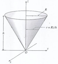
Find the moment of inertia tensor for a uniform solid cone of mass [math]M[/math] , height [math]h[/math] , and base radius [math]R[/math] spinning about its tip.

Choose the z-axis so it is along the symmetry axis of the cone.

The mass density may be written as

[math]\rho = \frac{M}{V}[/math]

Using cylindrical coordinates ( [math]r, \phi, z[/math]) the volume of a cone is given by

[math]V = \int_0^h dz \int _0^{2\pi}d\phi \int_0^{\frac{Rz}{h}} r dr = \int_0^h dz \int _0^{2\pi}d\phi \frac{R^2z^2}{2h^2}= 2 \pi \frac{R^2}{2h^2}\int_0^h z^2 dz [/math]

[math] = \pi \frac{R^2}{h^2} \frac{h^3}{3} =\frac{1}{3} \pi R^2 h [/math]

the radius of the base of the cone may be written as a function such that [math] r=\frac{Rz}{h}[/math] .

When [math]z=0 \Rightarrow r=0[/math] and when [math]z=h \Rightarrow r = R[/math]

[math]\rho = \frac{M}{V} = \frac{M}{\frac{1}{3} \pi R^2 h} = \frac{ 3 M}{\pi R^2 h} [/math]

calculating the moment of inertia about the z-axis :

[math]I_{zz} = \int \rho \left (x^2+y^2 \right ) dV= \int_0^h \int _o^{2\pi} \int_0^{\frac{Rz}{h}} \rho r^2 r dr d\phi dz[/math]

[math]I_{zz} = \rho \int_0^h dz \int _0^{2\pi}d\phi \int_0^{\frac{Rz}{h}} r^2 r dr [/math]

[math] = \rho \int_0^h dz (2 \pi) \frac{R^4z^4}{4h^4} [/math]

[math] = 2 \pi \rho \frac{R^4}{4h^4}\int_0^h z^4 dz [/math]

[math] = 2 \pi \rho \frac{R^4}{4h^4} \frac{h^5}{5} [/math]

[math] = 2 \pi \left ( \frac{ 3 M}{\pi R^2 h}\right ) \frac{R^4}{4h^4} \frac{h^5}{5} [/math]

[math] = 3 M \frac{R^2}{2h^5} \frac{h^5}{5} = \frac{3}{10} M R^2 [/math]

[math]I_{xx} = \int \rho \left (z^2+y^2 \right ) dV= \int \rho z^2 dV +\int \rho y^2 dV[/math]

Since

[math]I_{zz} = \int \rho \left (x^2+y^2 \right ) dV[/math]

and the cone is symmetric in the x-y plane

[math]\int \rho y^2 dV = \frac{1}{2} I+{zz}[/math]

[math] \int \rho z^2 dV = \rho \int_0^h z^2 dz \int _0^{2\pi}d\phi \int_0^{\frac{Rz}{h}} r dr = 2 \pi \rho \int_0^h z^2 dz \frac{R^2z^2}{2h^2} [/math]

[math] = \pi \rho \frac{R^2}{h^2}\int_0^h z^4 dz = \pi \rho \frac{R^2}{h^2} \frac{h^5}{5} [/math]

[math] = \pi \left ( \frac{ 3 M}{\pi R^2 h}\right ) frac{R^2h^3}{5} = \frac{3Mh^2}{5} [/math]

[math]I_{xx} =\frac{3}{20} M R^2 + \frac{3Mh^2}{5}[/math]

[math]I_{yy } = \int \rho \left (z^2+x^2 \right ) dV = \frac{3}{20} M R^2 + \frac{3Mh^2}{5}= \frac{3}{20} M \left ( R^2 + 4h^2 \right ) = I_{xx}[/math]

The products of inertia

Product of Inertia of a rigid body that relates the x(y) component of the angular momentum for rotations about the y(x)-axis

[math]I_{xy} \equiv \sum m_k(-x_{k} y_{k}) =\int \rho xy dV[/math]

From the viewpoint of the summation equation one can see that for every mass at point (x,z) there is an equal mass at the point (-x,z), Thus the sum will add to zero.

or mathematically

[math]I_{xy} =\int \rho xy dV =\int_0^h dz \int _0^{2\pi}d\phi \int_0^{\frac{Rz}{h}} r dr \rho xy =\int_0^h dz \int _0^{2\pi}d\phi \int_0^{\frac{Rz}{h}} r dr \rho (r \cos \phi ) ( r \sin \phi) [/math]

[math]=\rho \int_0^h dz \int _0^{2\pi}d\phi \cos \phi \sin \phi \int_0^{\frac{Rz}{h}} r^3 dr [/math]

[math]\int _0^{2\pi}d\phi \cos \phi \sin \phi =\int _0^{2\pi} \sin \phi d(\sin \phi) = \left . \frac{1}{2}\sin^2 \phi \right |_{0}^{2\pi} = 0 [/math]

Product of Inertia of a rigid body that relates the x(z) component of the angular momentum for rotations about the z(x)-axis

[math]I_{xz} \equiv \sum m_k(-x_{k} y_{k}) =-\int \rho xz dV [/math]

[math]= -\int_0^h dz \int _0^{2\pi}d\phi \int_0^{\frac{Rz}{h}} r dr \rho r \cos \phi z= -\rho \int_0^h z dz \int _0^{2\pi} \cos \phi d\phi \int_0^{\frac{Rz}{h}} r^2 dr [/math]

Product of Inertia of a rigid body that relates the y(z) component of the angular momentum for rotations about the y(x)-axis

[math]I_{yz} \equiv \sum m_k \left (-y_{k} z_{k} \right ) [/math]

[math]=-\int \rho yz dV = -\int_0^h dz \int _0^{2\pi}d\phi \int_0^{\frac{Rz}{h}} r dr \rho r \sin \phi z= -\rho \int_0^h z dz \int _0^{2\pi} \sin \phi d\phi \int_0^{\frac{Rz}{h}} r^2 dr [/math]

[math]\int _0^{2\pi} \sin \phi d\phi =\int _0^{2\pi} \cos \phi d\phi = 0[/math]

If the inertia tensor is diagonal (off diagnonal elements are zero)

Then The angular momentum points in the same direction as the angular velocity.

[math] I = \frac{3}{20} M \left( \begin{array}{ccc} R^2+4h^2 & 0 & 0\\ 0 & R^2+4h^2 & 0 \\0 & 0 & 2R^2 \end{array} \right) [/math]

http://scienceworld.wolfram.com/physics/MomentofInertiaSphere.html

http://www.phys.ufl.edu/~mueller/PHY2048/2048_Chapter10_F08_Part2_lecture.pdf

Precession of a Top

As shown above,the angular momentum tensor of a top rotating about its axis of symmetry with respect to its tip is

[math] I = \frac{3}{20} M \left( \begin{array}{ccc} R^2+4h^2 & 0 & 0\\ 0 & R^2+4h^2 & 0 \\0 & 0 & 2R^2 \end{array} \right) \equiv \left( \begin{array}{ccc} \lambda_1 & 0 & 0\\ 0 & \lambda_2 & 0 \\0 & 0 & \lambda_3\end{array} \right) [/math]

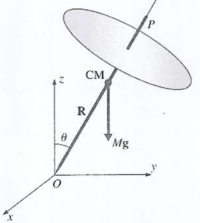
Suppose the top make a small angle [math]\theta[/math] with respect to the normal of the surface it is spinning on top of.

[math]\vec F = M g \hat k[/math]

The resulting torque from this gravitational force is

[math]\vec \tau = \vec R \times M \vec g = \vec \dot L \;\;\;\; \Rightarrow \;\;\;\; \left | \vec \tau \right | = Mg \sin \theta [/math]

where [math]\vec R[/math] is a vector pointing to top's center of mass from the principal axes that make up a coordinate system whose origin is at the tip of the top

[math]\vec R = R \hat k[/math]

[math]\vec g = -g \hat z[/math] ( [math]\hat z[/math] points normal to the surface that the top is spinning on)

Initially the angular velocity ( and angular momentum) are pointed along the [math]\hat k[/math] principal axis.

[math]\vec L = \lambda_2 \omega \hat k[/math]

Newton's second law for the angular motion [math]\Rightarrow[/math]

[math]\vec \tau = \vec \dot L[/math]

[math] \vec R \times M \vec g = \lambda_2 \omega \hat \dot k[/math]

[math] R \hat k \times M g \hat z = \lambda_2 \omega \hat \dot k[/math]

[math] \frac{MgR}{\lambda_2 \omega} \hat k \times \hat z = \hat \dot k[/math]

Let

[math] \vec \Omega = \frac{MgR}{\lambda_2 \omega} \hat k[/math] = precession frequency of the top

The axis of the top [math]\hat k[/math] rotates with an angular speed [math]\Omega[/math] about the [math]\hat z[/math] axis.

The direction of the external torque [math] \vec R \times \vec g[/math] is in the [math]- \hat i[/math] direction at the instant shown in the above figure. As a result the top will rotate in the counter-clockwise direction about the z-axis as viewed from above the z-axis.

Principal Axis

As seen in the case of a precessing top above, the physics of a rotating rigid body can be more easily described when the inertia tensor is diagonal. One need only find a coordinate system in which the tensor is diagonal in order to simplify the problem.

Principal axis

The axis of rotation for a rigid body in which the moment of inertia tensor is diagonal thereby the Angular momentum will be parallel to the angular velocity.

In the above example of the top ( solid cone), the x,y, and z axes of the chosen coordinate system are principal axes of inertia and the moments of inertia are the principal moments.

One can observe from the example of a spinning top, that a rotation axis around which the rigid body is symmetry will tend to be a principal axis.

Additionally, if the body has two perpendicular planes of reflection symmetry, then the three perpendicular axes defined by these two planes and a point of rotation are principal axes.

Existence of Principal Axes

Although it is easy to see which are the principal axes when the rigid body is symmetric, it is true that any rigid body's rotating about a point has three principal axes.

Finding the Principal axis of a Rigid body

Once the Inertia tensor is known, the principal axes of a rigid body may be found by "diagonalizing" the tensor matrix.

The process of "diagonalizing" the tensor matrix amounts to solving an eigenvalue problem.

The angular momentum of a rigid body can be given by

[math]\vec L = \tilde{I} \vec \omega[/math]

For the special case that the angular momentum (\vec L) is parallel to the angular velocity (\vec \omega)

Then

[math]\vec L = \lambda \vec \omega[/math]

To determine the principal axes you determine the vector [math]\vec omega[/math] such that

[math]\tilde I \vec \omega = \lambda \vec \omega[/math]

In practice, one determines [math]\vec \omega[/math] ( the eigen vectors) by solving for [math]\lambda[/math] (the eigenvalues) such that

[math]\left (\tilde I- \lambda \tilde 1 \right ) \vec \omega =0[/math]

where

[math] \tilde 1 \equiv \left( \begin{array}{ccc}1 & 0 & 0\\ 0 & 1 & 0 \\0 & 0 & 1\end{array} \right) [/math] = unit matrix

In order for the above matrix problem (system of 3 equations and 3 unknowns) to have a non-zero solution the secular equation must hold ( the determinant must be non-zero)

[math]det \left (\tilde I- \lambda \tilde 1 \right ) \equiv \left |\tilde I- \lambda \tilde 1 \right | =0[/math]

One solves the above equation by first finding the three eigenvalues that will make the above determinant zero and then use Gauss-Jordan elimination of the augmented matrix using each of the eigenvalues separately to find the eigenvector for that particular eigenvalue

For example:

Suppose the momentum tensor is given by

[math] \tilde I \equiv \left( \begin{array}{ccc}8 & -3 & -3\\ -3 & 8 & -3 \\-3 & -3 & 8\end{array} \right) [/math]

[math]\left |\tilde I- \lambda \tilde 1 \right | =0[/math]

[math] \left |\begin{array}{ccc}8-\lambda & -3 & -3\\ -3 & 8-\lambda & -3 \\-3 & -3 & 8-\lambda\end{array} \right | =0[/math]

[math]\Rightarrow[/math]

[math](2-\lambda)(11-\lambda)^2 =0[/math]

[math]\Rightarrow \;\;\; [/math] 3 solutions [math]\lambda_1 = 2 \;\;\;\;\lambda_2=\lambda_3 = 11[/math]

You can find the eigenvector for each eigenvalue by performing Gauss-Jordan row-column reduction of the augmented matrix

for the eigenvalue [math] \lambda_1 = 2[/math]

[math]\left (\tilde I- 2 \tilde 1 \right ) \vec \omega =0[/math]

[math] \left (\begin{array}{ccc}8-2 & -3 & -3\\ -3 & 8-2 & -3 \\-3 & -3 & 8-2\end{array} \right ) \vec \omega =0[/math]

[math] \left (\begin{array}{ccc}6 & -3 & -3\\ -3 & 6 & -3 \\-3 & -3 & 6\end{array} \right ) \vec \omega =0[/math]

In augmented form:

[math] \left (\begin{array}{cccc}6 & -3 & -3 & 0 \\ -3 & 6 & -3 & 0\\-3 & -3 & 6& 0\end{array} \right ) [/math]

Divide everything by 3

[math] \left (\begin{array}{cccc}2 & -1 & -1 & 0 \\ -1 & 2 & -1 & 0\\-1 & -1 & 2& 0\end{array} \right ) [/math]

Add the second row to the first row

[math] \left (\begin{array}{cccc}1 & 1 & -2 & 0 \\ -1 & 2 & -1 & 0\\-1 & -1 & 2& 0\end{array} \right ) [/math]

Add the first row to the second and third row

[math] \left (\begin{array}{cccc}1 & 1 & -2 & 0 \\ 0 & 3 & -3 & 0\\0 & 0 & 0& 0\end{array} \right ) [/math]

Divide the second row by 3

[math] \left (\begin{array}{cccc}1 & 1 & -2 & 0 \\ 0 & 1 & -1 & 0\\0 & 0 & 0& 0\end{array} \right ) [/math]

Subtract the first row by the second row

[math] \left (\begin{array}{cccc}1 & 0 & -1 & 0 \\ 0 & 1 & -1 & 0\\0 & 0 & 0& 0\end{array} \right ) [/math]

The above augmented matrix represents the following system of equations

row 1 : [math]\omega_x - \omega_z = 0[/math]

row 2 : [math]\omega_y - \omega_z = 0[/math]

row 1 : [math]0 * \omega_z = 0 \Rightarrow \;\;\; \omega_3[/math] is arbitary

thus

[math]\omega_x=\omega_y= \omega_z [/math]

[math]\hat e_1 = \hat i + \hat j + \hat k[/math]

but the above needs to be a unit vector such that

[math]\hat e_1 \cdot \hat e_1 = 1[/math]

therefor

[math]\hat e_1 = \frac{1}{\sqrt{3}} \left ( \hat i + \hat j + \hat k\right )[/math]

for the eigenvalue [math] \lambda_2 = 11[/math]

[math]\left (\tilde I- 2 \tilde 1 \right ) \vec \omega =0[/math]

[math] \left (\begin{array}{ccc}-3 & -3 & -3\\ -3 & -3 & -3 \\-3 & -3 & -3\end{array} \right ) \vec \omega =0[/math]

[math](\tilde I - \lambda_2 \tilde 1 ) \vec \omega = \left (\begin{array}{ccc}-3 & -3 & -3\\ -3 & -3 & -3 \\-3 & -3 & -3\end{array} \right )\left (\begin{array}{c} \omega_x \\ \omega_y \\ \omega_z \\ \end{array} \right ) =0[/math]

[math]\Rightarrow \omega_x + \omega_y + \omega_z = 0[/math]

All three components of [math]\omega[/math] add up to zero or in other words

[math] \omega_x + \omega_y + \omega_z = \vec \omega \cdot \hat e_1 = 0 0[/math]

The remaining two principal axis must be perpendicular to the principal axis with eigenvalue [math]\lambda_1 =2[/math].

Otherwise the remaining two principal axes are arbitrary and indicate that the rigid body is symmetric about these two remaining axes.

BTW: The above moment of inertia represents the moment of inertia of a cube rotating about one of its corners. The principal axis [math]\hat e_1[/math] is a vector that traverses the diagonal of the cube.

Euler's Equations

Space Frame and Body Frame

Space Frame

An inertial reference frame used to locate the center of mass of a rigid body [math](\hat i , \hat j, \hat k)[/math]

Body Frame

A non-inertial reference frame that uses the principal axes of a rotating rigid body [math](\hat e_1 , \hat e_2, \hat e_3)[/math]

.

If a body has an angular momentum [math]\vec \omega[/math] and principal moments [math]\lambda_1 ,\lambda_2[/math] and [math]\lambda_3[/math]

Then the angular momentum [math]\vec L[/math] in the Body reference frame is given by

[math]\left (\vec L \right )_{\mbox{Body}} = \tilde I \vec \omega = \left (\begin{array}{ccc}\lambda_1 & 0 & 0\\ 0 & \lambda_2 & 0 \\0 & 0 & \lambda_3\end{array} \right )\left (\begin{array}{c} \omega_x \\ \omega_y \\ \omega_z \\ \end{array} \right ) = \lambda_1 \omega_1 \hat e_1 +\lambda_2 \omega_2 \hat e_2 +\lambda_3 \omega_3 \hat e_3= \sum \lambda_i \omega_i \hat e_i[/math]

The torque in the Space reference frame is given by

[math]\vec \tau = \frac{d}{dt} \left (\vec L \right )_{\mbox{Space}}[/math]

[math]\left (\vec L \right )_{\mbox{Body}}[/math] is moving as seen in the Space frame

[math] \frac{d}{dt} \left (\vec L \right )_{\mbox{Space}} = \frac{d}{dt} \left (\sum \lambda_i \omega_i \hat e_i \right )_{\mbox{Body}}[/math]

[math] = \left (\sum \frac{d\lambda_i \omega_i}{dt} \hat e_i \right )_{\mbox{Body}} + \sum \lambda_i \omega_i\left (\frac{d\hat e_i }{dt} \right )_{\mbox{space}}[/math]

remembering that

[math]\vec v = \vec \omega \times \vec r[/math]

one can see that

[math]\frac{ d \hat e_i}{dt} = \omega \times \hat e_i[/math]

[math] \vec \tau=\frac{d}{dt} \left (\vec L \right )_{\mbox{Space}} = \left (\vec \dot L\right )_{\mbox{Body}} + \vec \omega \times \vec L[/math] : Euler's equation

[math] = \left (\vec \dot L\right )_{\mbox{Body}} + \left (\begin{array}{ccc}\hat e_1 & \hat e_2 & \hat e_3 \\ \omega_1 & \omega_2 & \omega_3 \\\lambda_1\omega_1 & \lambda_2\omega_2 & \lambda_3\omega_3\end{array} \right )[/math]

Euler's equation for the spinning top

In the case of the spinning top:

The external torque applied by gravity is always normal to the z-axis ([math]\hat e_3[/math]) so value of the torque is zero in the [math]\hat e_3[/math] direction

[math]\Rightarrow \;\;\;\; \lambda_3 \dot \omega_3 - ( \lambda_1-\lambda_2)\omega_1 \omega_2 = 0[/math]

but

[math]\lambda_1=\lambda_2[/math]

so

[math] \lambda_3 \dot \omega_3 = 0 \Rightarrow[/math] the tops angular velocity along the symmetry axis is constant.

Euler's Equation for Zero Torque

[math]\vec \dot L = \left (\frac{d}{dt}\vec L \right )_{\mbox{Body}} = - \vec \omega \times \vec L[/math]

[math]= -\left (\begin{array}{ccc}\hat e_1 & \hat e_2 & \hat e_3 \\ \omega_1 & \omega_2 & \omega_3 \\\lambda_1\omega_1 & \lambda_2\omega_2 & \lambda_3\omega_3\end{array} \right )[/math]

Two principal moments are the same value (Free precession)

The motion of a top is an example of this situation. As seen above for the motion of the top,

[math]\tau_3= \lambda_3 \dot \omega_3 - ( \lambda_1-\lambda_2)\omega_1 \omega_2 = 0[/math] The torque is alway zero in the z-direction [math](\hat e_3)[/math]

[math]\lambda_3 \dot \omega_3 =0 \;\;\;\; \Rightarrow \omega_3 =[/math] constant

The remaining Euler equations are

[math]\tau_1= \lambda_1 \dot \omega_1 - ( \lambda_2-\lambda_3)\omega_2 \omega_3[/math]

[math]\tau_2= \lambda_2 \dot \omega_2 - ( \lambda_3-\lambda_1)\omega_1 \omega_3[/math]

IF the top is aligned with the z-axis then there will be no torque. (But as soon as it is misaligned there will be a torque)

The above Euler equations become

[math] \lambda_1 \dot \omega_1 = \left [ ( \lambda_2-\lambda_3)\omega_3\right ] \omega_2 = \left [ ( \lambda-\lambda_3)\omega_3\right ] \omega_2 [/math]

[math] \lambda_2 \dot \omega_2 = \left [( \lambda_3-\lambda_1)\omega_3\right ] \omega_1 = -\left [( \lambda-\lambda_3)\omega_3\right ] \omega_1 [/math]

where

[math]\lambda=-\lambda_1=\lambda_2[/math]

let

[math]\Omega_b \equiv \frac{\lambda-\lambda_3}{\lambda}\omega_3[/math] = angular frequency of the body cone

The we as a coupled set of equations as we saw before

[math] \dot \omega_1 = \Omega_b \omega_2 [/math]

[math] \dot \omega_2 = -\Omega_b \omega_1 [/math]

using the trick of defining a complex frequency such that

[math]\zeta = \omega_1 + i \omega_2[/math]

Forest_Ugrad_ClassicalMechanics#Rigid_Body_Motion