Forest UCM MiNF

Mechanics in Noninertial Reference Frames

Linearly accelerating reference frames

Let [math]\mathcal S_0[/math] represent an inertial reference frame and [math]\mathcal S[/math] represent an noninertial reference frame with acceleration [math]\vec A[/math] relative to [math]\mathcal S_0[/math].

Ball thrown straight up

Consider the motion of a ball thrown straight up as viewed from [math]\mathcal S[/math].

Using a Galilean transformation (not a relativistic Lorentz transformation)

At some instant in time the velocities add like

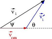
[math]\dot {\vec {r}_0} = \dot {\vec r}+ \vec V[/math]

where

[math]\vec V[/math] = velocity of moving frame [math]\mathcal S[/math] with respect to [math]\mathcal S_0[/math] at some instant in time

[math]\Rightarrow \dot {\vec r} = \dot {\vec {r}_0} - \vec V[/math]

taking derivative with respect to time

[math]\Rightarrow \ddot {\vec r} = \ddot {\vec {r}_0} - \dot {\vec V} = \ddot {\vec {r}_0} - \vec A [/math]

[math]\Rightarrow m\ddot {\vec r} = m\ddot {\vec {r}_0} - m \vec A= \vec F - m\vec A= \vec F - \vec {F}_{\mbox {inertial}}[/math]

where

[math]\vec {F}_{\mbox {inertial}} = m \vec A \equiv[/math] inertial force

in your noninertial frame, the ball appears to have a force causing it to accelerate in the [math]\vec A[/math] direction.

The inertial force may also be referred to as a fictional force

an example is the "fictional" centrifugal force for rotational acceleration.

The observer in a noninertial reference frame will feel these frictional forces as if they are real but they are really a consequence of your accelerating reference frame

example

A force pushes you back into your seat when your Jet airplane takes off

you slam on the brakes and hit your head on the car's dashboard

Pedulum in an accelerating car

Consider a pendulum mounted inside a car that is accelerating to the right with a constant acceleration [math]\vec A[/math].

What is the pendulums equilibrium angle [math]\theta_0[/math]

In frame [math]\mathcal S_0[/math]

[math]\sum \vec F = m \ddot{\vec r_0}= \vec T + m \vec g[/math]

In frame [math]\mathcal S[/math]

[math]\sum \vec F = m \ddot{\vec r}= \vec T + m \vec g - m \vec A= \vec T + m \left ( \vec g -\vec A \right ) = \vec T + m \vec g_{eff} [/math]

If the pendulum is at rest and not oscillating then

[math]\sum \vec F = 0 = \vec T + m \vec g_{eff} [/math]

[math]g_{eff}[/math] is the vector sum of [math]g[/math] and [math]A[/math] which are orthogonal to each other in this problem thus

[math]\theta = \tan^{-1}{\frac{A}{g}}[/math]

The pendulum oscillation frequency as seen in the accelerating car is

[math]\omega= \sqrt{\frac{g_{eff}}{l}} = \sqrt{\frac{\sqrt{g^2+A^2}}{l}}[/math]

Using lagrangian mechanics in the inertial frame

[math]\vec{r} = (l \sin \theta + \frac{1}{2} a t^2) \hat i + l \cos \theta \hat j[/math]

[math]\dot {\vec{r}} = (l \cos \theta \dot {\theta} + a t ) \hat i + \sin \theta \dot {\theta} \hat j[/math]

[math] T = \frac{1}{2} mv^2 = \frac{1}{2} m \left ( (l \cos \theta \dot \theta + a t)^2 + \sin^2 \theta \dot \theta^2 \right )[/math]

[math]= \frac{1}{2} m \left ( l^2 \dot \theta^2 + 2 atl\dot \theta \cos \theta + a^2t^2\right )[/math]

[math]U =- mgy = -mgl \cos \theta[/math]

[math]\mathcal L = \frac{1}{2} m \left ( l^2 \dot \theta^2 + 2 atl\dot \theta \cos \theta + a^2t^2\right ) +mgl \cos \theta[/math]

[math] \left ( \frac{\partial \mathcal {L} }{\partial \theta} \right ) = \frac{d}{dt} \left ( \frac{\partial \mathcal {L} }{\partial \dot \theta} \right ) [/math]

[math] -matl \dot \theta \sin \theta -mgl\sin \theta = \frac{d}{dt} \left ( ml^2\dot \theta + matl \cos \theta \right ) [/math]

[math] -at \dot \theta\sin \theta -g\sin \theta = l\ddot \theta - at \sin \theta \dot \theta + a \cos \theta[/math]

[math] l\ddot \theta=-g\sin \theta + a \cos \theta [/math]

The tides view by a ref frame accelerating towards the moon

The gravitational force between the moon and the earth accelerates the earth towards the moon.

This makes the earth an accelerated reference frame

The moon of mass [math](M_m)[/math] pulls on the earth of mass [math](M_e)[/math] such that

[math]\vec F = G \frac{M_m M_e}{d_0^3}\vec d_0 = M_e \vec A[/math]

where [math]d_0[/math] is the earth-moon distance of separation.

[math]\Rightarrow \vec A = G \frac{M_m }{d_0^3}\vec d_0 =[/math] Earth's acceleration towards the moon that makes the earth a non-inertial reference frame

The moon of mass [math](M_m)[/math] pulls on a test mass of water [math](M_o)[/math] on the surface of the earth's ocean such that

[math]\vec F = G \frac{M_m M_o}{d^3}\vec d[/math]

As seen in the Earth non-inertial reference frame

[math]M_o \ddot {\vec r} = \sum \vec F - M_o \vec A[/math]

[math]= \left ( M_o \vec g + \vec F_N + G \frac{M_m M_o}{d^3}\vec d \right ) - G \frac{M_m }{d_0^3}\vec d_0 [/math]

where

[math]\vec F_N =[/math] a net non-graviational force hold the mass M_o in top of the ocean (Bouyant force)= M(dis0laced water)*g

[math] M_o \ddot \vec r = \left ( M_o \vec g + {\vec F}_N + G \frac{M_m M_o}{d^3} \vec d \right ) - G \frac{M_m }{d_0^3}\vec d_0 [/math]

[math]= M_o \vec g + \vec F_N + \vec{F}_{\mbox{tide}}[/math]

[math]\vec{F}_{\mbox{tide}} = G \frac{M_m M_o}{d^3}\vec d - G \frac{M_m }{d_0^3}\vec d_0 [/math]

[math] = G M_m M_o \left ( \frac{\vec d}{d^3} - \frac{\vec d_0}{d_0^3}\right ) [/math]

Let's consider two cases, one where M_o is directly between the moon and the earth and the other when the mass is directly on the opposite side of the earth from the moon.

Case 1

The mass is directly between the moon and the earth

In this case [math]\vec d || \vec d_0 [/math] and [math]d_0 \lt d[/math] making [math]\vec{F}_{\mbox{tide}}[/math] pull [math]M_o[/math] towards the moon

Case 2

The mass is directly on the other side of the earth with respect to the moon

In this case [math]\vec d || \vec d_0 [/math] BUT [math]d_0 \gt d[/math] making [math]\vec{F}_{\mbox{tide}}[/math] pull [math]M_o[/math] away from the moon

Magnitude of the Tides

Consider a drop of water of mass [math]m[/math] on the surface of the ocean.

The three forces influencing this drop from the previous sections are

[math]\vec F_g =M_o \vec g \;\;\;\; \vec{F}_{\mbox{tide}} \;\;\;\;\; \vec F_N[/math]

Archimedes Principle

An object in a fluid is buoyed up with a force equal to the weight of the water displaced by the object.

All of the above forces act normal to the surface of the water.

[math]\vec F_g = M_o \vec g \;\;\;\; \vec{F}_{\mbox{tide}} [/math]

are the result of a gravitational force which is conservative.

A potential may be defined for the two forces above such that

[math]\vec F_g = M_o \vec g = -\nabla U_{eg} \;\;\;\; \vec{F}_{\mbox{tide}} = - \nabla U_{\mbox{tide}} [/math]

[math]\vec{F}_{\mbox{tide}} = G \frac{M_m M_o}{d^3}\vec d - G \frac{M_m }{d_0^3}\vec d_0 \equiv - \nabla U_{\mbox{tide-1}}- \nabla U_{\mbox{tide-2}}[/math]

[math]G \frac{M_m M_o}{d^3}\vec d \equiv - \nabla U_{\mbox{tide-1}}[/math]

[math]\Rightarrow U_{\mbox{tide-1}}=G M_m M_o\frac{1}{d} \;\;\;\;\;[/math]:[math] \;\;\;\;\vec d[/math] is NOT always pointed along the x-axis towards the moon

[math] G \frac{M_m M_o}{d_0^3}\vec d_0 \equiv \nabla U_{\mbox{tide-2}}[/math]

[math] U_{\mbox{tide-2}} = - \int \vec F_o \cdot d \hat x= \int G \frac{M_m M_o }{d_0^2}\hat {d}_0 \cdot d \hat x[/math]

[math] = G \frac{M_m M_o}{d_0^2}\int\hat {d}_0 \cdot d \hat x[/math] Since [math]d_0[/math] is at fixed distance

[math] = G \frac{M_mM_o }{d_0^2}\int\ d x[/math] Since [math]d_0[/math] is parallel to x

[math] = G M_m M_o\frac{x}{d_0^2}[/math]

[math] U_{\mbox{tide}}=-G M_m M_o \left ( \frac{1}{d} + \frac{x}{d_0^2} \right ) [/math]

Since

[math]\vec F_g = M_o \vec g = -\nabla U_{eg} \;\;\;\; \vec{F}_{\mbox{tide}} = - \nabla U_{\mbox{tide}} [/math]

are forces that are exerted such that the are always perpendicular to the surface of the ocean ( they are normal to the surface) then the sum of the two potential's, [math]U_{eg} + U_{\mbox{tide}}[/math], is constant on the surface

[math]\Rightarrow[/math] The ocean's surface is an equipotential surface ( all points on the surface of the ocean are have the same gravitational potential energy

If you consider two points on the surface of the earth where one point is high tide (HT) and the other point is low tide (LT) then

[math]U_{eg}(HT) + U_{\mbox{tide}}(HT)=U_{eg}(LT) + U_{\mbox{tide}}(LT)[/math]

The change in the gravitational potential energy between the earth and the ocean for high tide and low tide is

[math]M_o gh=U_{eg}(HT)-U_{eg}(LT)[/math]

but

[math]U_{eg}(HT) -U_{eg}(LT)= U_{\mbox{tide}}(LT) - U_{\mbox{tide}}(HT)[/math]

[math]M_ogh= -G M_m M_o \left ( \frac{1}{\sqrt{d_0^2+r^2}} + \frac{0}{d_0^2} \right )- (-G M_m M_o) \left ( \frac{1}{d_0-R_e} + \frac{-R_e}{d_0^2} \right ) [/math]

At HT

[math]d = d_0 - R_e \;\;\;\; x = -R_e[/math]

At LT

[math]d = \sqrt{d_0^2 + r^2} \;\;\;\; x = 0[/math]

[math]\frac{1}{\sqrt{d_0^2+r^2}} \approx \frac{1}{\sqrt{d_0^2+R_e^2}} = \frac{1}{d_0 \sqrt{1 + \left ( \frac{R_e}{d_0} \right )^2}} \approx\frac{1}{d_0} \left ( 1 - \frac{1}{2} \left ( \frac{R_e}{d_0} \right )^2 \right ) [/math]

[math]M_ogh= -G M_m M_o \left [ \left ( \frac{1}{\sqrt{d_0^2+r^2}} \right )- \left ( \frac{1}{d_0-R_e} + \frac{-R_e}{d_0^2} \right ) \right ][/math]

[math]= -G M_m M_o \left [ \frac{1}{d_0} \left ( 1 - \frac{1}{2} \left ( \frac{R_e}{d_0} \right )^2 \right ) - \left ( \frac{1}{d_0-R_e} + \frac{-R_e}{d_0^2} \right ) \right ][/math]

[math]= -G M_m M_o \left [ \frac{1}{d_0} \left ( 1 - \frac{1}{2} \left ( \frac{R_e}{d_0} \right )^2 \right ) - \frac{1}{d_0}\left ( \frac{1}{1-\frac{R_e}{d_0}} + \frac{-R_e}{d_0^2} \right ) \right ][/math]

[math]\frac{1}{1-x} = 1 + x + x^2 = \sum_n^{\infty} x^n[/math] : geometric series when[math] x \lt 1[/math]

[math]M_o gh= -G M_m M_o \left [ \frac{1}{d_0} \left ( 1 - \frac{1}{2} \left ( \frac{R_e}{d_0} \right )^2 \right ) - \frac{1}{d_0}\left (1 + \frac{R_e}{d_0} + \left( \frac{R_e}{d_0} \right)^2 - \frac{R_e}{d_0^2} \right ) \right ][/math]

[math] -G M_m M_o \left [ \frac{1}{d_0} \left ( 1 - \frac{1}{2} \left ( \frac{R_e}{d_0} \right )^2 \right ) - \frac{1}{d_0}\left (1 + \left( \frac{R_e}{d_0} \right)^2 \right ) \right ][/math]

[math] -G M_m M_o \left [ \frac{1}{d_0} \left ( - \frac{3}{2} \left ( \frac{R_e}{d_0} \right )^2 \right ) \right ][/math]

[math] \frac{G M_m M_o}{d_o} \left [ \frac{3}{2} \left ( \frac{R_e}{d_0} \right )^2 \right ][/math]

[math]g = G\frac{M_e}{R_e^2}[/math]

[math]M_o gh=\frac{G M_m M_o}{d_o} \left [ \frac{3}{2} \left ( \frac{R_e}{d_0} \right )^2 \right ][/math]

[math]M_o \left ( G\frac{M_e}{R_e^2} \right) h=\frac{G M_m M_o}{d_o} \left [ \frac{3}{2} \left ( \frac{R_e}{d_0} \right )^2 \right ][/math]

[math] h= \frac{3}{2} \frac{ M_m R_e^4}{M_ed_o^3}[/math]

Height of Tides due to Moon and Sun

[math] h= \frac{3}{2} \frac{ M_m R_e^4}{M_ed_o^3}[/math]

[math] M_m = 7.35 \times 10^{22}[/math] kg = mass of moon

[math] M_e = 5.98 \times 10^{24}[/math] kg = mass of earth

[math] M_s = 1.99 \times 10^{30}[/math] kg = mass of sun

[math] R_e = 6.37 \times 10^{6}[/math] m

[math]d_m = 3.84 \times 10^{8}[/math] m = earth-moon distance

[math]h= 54 cm =[/math] height of tides due to the moon

[math] d_s = 1.495 \times 10^{11}[/math] m = earth-sun distance

[math]h = 25 cm =[/math] height of tides due to sun

spring tides

The case when the moon, earth and sun are aligned to give maximum height tide (moon can be either full or new doesn't matter because the bulge is on both sides of the earth)

neap tides

This is the case then the sun, earth, and sun are aligned to form a right triangle. The tide effect should cancel so the height is only 54-25=29 cm.

Euler's Theorem of rotation

Original form:

Any displacement of a rigid body in three dimensional space such that a point on the rigid body, say O, remains fixed, is equivalent to a rotation about a fixed axis through the point O.

Expressed using Modern mathematical terms

Euler's theorem on the axis of a three dimensional rotation

If [math]\mathbf{R}[/math] is a 3x3 orthogonal matrix [math](\mathbf{R}^T\mathbf{R} = \mathbf{RR}^T = 1)[/math] and [math]\mathbf R[/math] is proper [math]( \left | \mathbf{R} \right | = +1) [/math], then there is a non-zero vector [math]r[/math] such that [math]\mathbf {R}r = r[/math]

The matrix R above represents a spatial rotation that is a linear one-to-one mapping that transforms the coordinate vector P into p.

The above theorem can be proven by treating it as a matrix algebra problem where you want to prove. ie

[math]\mathbf {R} \vec P = \lambda \vec p[/math]

First let's find the eigenvalues and eigenvectors of the matrix [math]\mathbf R[/math]

A consequence of Euler's theorem is that a single rotation may be represented as a combination of rotation.

Angular velocity vector

If we denote the angular velocity vector describing the angular velocity of a rotating body as [math]\omega[/math] the the magnitude and direction of this vector may be expressed as

[math]\vec \omega = \left | \vec \omega \right | \hat \omega[/math]

[math]\left | \vec \omega \right | \equiv[/math] magnitude of the rate of rotation (angular speed)

[math] \hat \omega \equiv[/math] direction of the rotation axis which is given by the right-hand rule and may is expressed using the components of a right handed coordinate system ( ie [math]\hat i,\hat j ,\hat k[/math] or [math]\hat r,\hat \theta,\hat \phi \cdots[/math])

[math]\vec \omega \equiv[/math] the angular velocity vector describing the angular velocity of a rotating body

[math]\vec \Omega \equiv[/math] The angular velocity vector describing the angular velocity of a rotating non-inertial reference frame.

Linear velocity from angular velocity

[math] \vec v = \vec \omega \times \vec r[/math] = linear velocity of a point located at the position [math]\vec r[/math] on a body rotating about the origin of the coordinate system used to specify [math]\vec r[/math].

Angular velocity addition

Consider two coordinate systems where [math]\mathcal S_0[/math] represent an inertial reference frame and [math]\mathcal S[/math] represent a frame with a velocity [math]\vec v[/math] relative to [math]\mathcal S_0[/math].

Using a Galilean transformation (not a relativistic Lorentz transformation)

the velocity [math]\vec v_{\mathcal S}[/math] in the moving frame [math]\mathcal S[/math] may be expressed in terms of the velocity [math]\vec v_{\mathcal S_0}[/math] in the rest frame and the velocity [math]u[/math] of the moving frame as.

[math]\vec v_{\mathcal S}=\vec v_{\mathcal S_0} - u [/math]

Now consider the situation when an object is rotating. The relationship between angular and linear motion should still satisfy the general express

[math]\vec v = \vec \omega \times \vec r[/math]

A point on this rotating body located by the position vector [math]\vec r[/math] from the inertial reference frame [math]\mathcal S_0[/math] will have the linear velocity

[math]\vec v_{\mathcal S_0} = \vec \omega_{\mathcal S_0} \times \vec r[/math]

If we fix a moving reference frame [math]\mathcal S[/math] so its origin coincides with [math]\mathcal S_0[/math] then the position of the same point on the object is given by the same position vector [math]\vec r[/math]. The angular velocity of this point is given by

[math]\vec v_{\mathcal S} = \vec \omega_{\mathcal S} \times \vec r[/math]

If the moving reference frame [math]\mathcal S[/math] is rotating with an angular velocity [math]\omega[/math] then the point on the object located by the vector [math]\vec r[/math] is moving with a linear velocity as viewed by [math]\mathcal S_0[/math] of

[math]\vec u = \vec \omega \times \vec r[/math]

Both the linear and the angular velocities add

[math]\vec v_{\mathcal S}=\vec v_{\mathcal S_0} - u [/math]

[math]\vec \omega_{\mathcal S} \times \vec r =\vec \omega_{\mathcal S_0} \times \vec r - \vec \omega \times \vec r[/math]

[math]=(\vec \omega_{\mathcal S_0} - \vec \omega ) \times \vec r[/math]

[math]\vec \omega_{\mathcal S}=(\vec \omega_{\mathcal S_0} - \vec \omega ) [/math]

Time derivative in Rotating Frame

Nomenclature

The following variables are used to describe the kinematics of a rotating frame

[math]\vec \mathbf V =[/math] linear velocity of the rotating frame

[math]\vec \mathbf A =[/math] linear acceleration of the rotating frame

[math]\vec \mathbf \Omega =[/math] angular velocity of the rotating frame

For example; a reference frame fixed to the earth with its origin at the center of the earth would be rotating with respect to an inertial frame with its origin at the same location with an angular velocity of one revolution every 24 hours.

[math]\mathbf \Omega = \frac{ 2 \pi \mbox {radians}}{24 \times 3600 \mbox{seconds}} = 7.3 \times 10^{-5} \frac{\mbox {rad}}{ \mbox{s}}[/math]

Rate of change of a general vector Q

let

[math]\vec \mathbf Q =[/math] an arbitrary vector representing position

Let's write the vector in terms of three orthonormal unit vectors representing an arbitrary right-handed coordinate system

[math]\vec \mathbf Q = \sum_{i=1}^3 Q_i \hat{e}_i = Q_1 \hat e_1 + Q_2 \hat e_2 + Q_3 \hat e_3 [/math]

[math]\left ( \frac{d \vec \mathbf Q}{dt}\right )_{\mathcal S}[/math] = rate of change of [math]\vec \mathbf Q[/math] as described by (relative to ) the rotating frame [math]\mathcal S[/math]

Using unit vectors that are attached to the rotating frame [math]\mathcal S[/math]

[math]\left ( \frac{d \vec \mathbf Q}{dt}\right )_{\mathcal S}=\left ( \frac{d }{dt} \sum_{i=1}^3 Q_i \hat{e}_i\right )_{\mathcal S}[/math]

[math]=\sum_{i=1}^3 \left ( \frac{d Q_i }{dt} \hat{e}_i + Q_i \frac{d \hat{e}_i }{dt} \right )_{\mathcal S}[/math]

In a cartesian coordinate system [math]\frac{d \hat{e}_i }{dt}=0 [/math]

[math]\left ( \frac{d \vec \mathbf Q}{dt}\right )_{\mathcal S}=\sum_{i=1}^3 \left ( \frac{d Q_i }{dt} \hat{e}_i \right )_{\mathcal S}[/math]

From the inertial reference frame [math]\mathcal S_0[/math] the above unit vectors used by [math]\mathcal S[/math] are changing their direction with time

[math]\left ( \frac{d \vec \mathbf Q}{dt}\right )_{\mathcal S_0}=\left ( \frac{d }{dt} \sum_{i=1}^3 Q_i \hat{e}_i\right )_{\mathcal S_0}[/math]

[math]=\sum_{i=1}^3 \left ( \frac{d Q_i }{dt} \hat{e}_i + Q_i \frac{d \hat{e}_i }{dt} \right )_{\mathcal S_0}[/math]

[math]=\sum_{i=1}^3 \left ( \frac{d Q_i }{dt} \hat{e}_i\right )_{\mathcal S_0} + \left ( Q_i \frac{d \hat{e}_i }{dt} \right )_{\mathcal S_0}[/math]

[math]\left ( \frac{d Q_i }{dt} \hat{e}_i\right )_{\mathcal S_0} =\left ( \frac{d Q_i }{dt} \hat{e}_i\right )_{\mathcal S} \equiv \frac{d Q_i }{dt} \hat{e}_i[/math] The expansion coefficients (vector components) of the vector are the same in both frames as the moving frames is not moving fast enough to be relativistic

[math] \left ( Q_i \frac{d \hat{e}_i }{dt} \right )_{\mathcal S_0}= Q_i \left ( \vec \mathbf \omega \times \hat e_i \right ) [/math] as seen earlier [math]\vec v = \frac{d \vec r}{dt} = \vec \omega \times \vec r[/math]

[math]\left ( \frac{d \vec \mathbf Q}{dt}\right )_{\mathcal S_0}=\sum_{i=1}^3 \left ( \frac{d Q_i }{dt} \hat{e}_i\right )_{\mathcal S_0} + \left ( Q_i \frac{d \hat{e}_i }{dt} \right )_{\mathcal S_0}[/math]

[math]=\sum_{i=1}^3 \frac{d Q_i }{dt} \hat{e}_i + Q_i \vec \mathbf \omega \times Q_i \hat e_i[/math]

[math]= \frac{d \vec \mathbf Q }{dt} + \vec \mathbf \omega \times \vec \mathbf Q[/math]

[math]= \left ( \frac{d \vec \mathbf Q }{dt} \right )_{\mathcal S} + \vec \mathbf \omega \times \vec \mathbf Q[/math]

The time derivative of a vector [math]\vec \mathbf Q[/math] as measured in the inertial frame [math]\mathcal S_0[/math] is related to the derivative in the non-inertial frame [math]\mathcal S[/math] by

[math]\left ( \frac{d \vec \mathbf Q}{dt}\right )_{\mathcal S_0}= \left ( \frac{d \vec \mathbf Q }{dt}\right )_{\mathcal S} + \vec \mathbf \omega \times \vec \mathbf Q[/math]

Newton's second law in a rotating frame

Newton's 2nd law in an inertial reference fram [math]\mathcal S_0[/math]

[math]\Rightarrow \sum \vec F = m \vec a_{\mathcal S_0} = m \left ( \frac{d^2 \vec r}{dt^2}\right )_{\mathcal S_0}[/math]

To determine the second derivative in a non-inertial frame we can take the derivative of the velocity relationship

[math]\left ( \frac{d^2 \vec r}{dt^2}\right )_{\mathcal S_0}=\left ( \frac{d }{dt}\right )_{\mathcal S_0}\left ( \frac{d \vec r}{dt}\right )_{\mathcal S_0}[/math]

[math]=\left ( \frac{d }{dt}\right )_{\mathcal S_0} \left [ \left ( \frac{d \vec r }{dt}\right )_{\mathcal S} + \vec \mathbf \Omega \times \vec r \right ][/math]

let

[math]\vec \mathbf Q \equiv \left [ \left ( \frac{d \vec r }{dt}\right )_{\mathcal S} + \vec \mathbf \Omega \times \vec r \right ][/math]

then

[math]\left ( \frac{d^2 \vec r}{dt^2}\right )_{\mathcal S_0}=\left ( \frac{d }{dt}\right )_{\mathcal S_0} \vec \mathbf Q[/math]

[math]\left ( \frac{d \vec \mathbf Q}{dt} \right )_{\mathcal S} + \vec \mathbf \Omega \times \vec \mathbf Q[/math]

[math]\left ( \frac{d \left [ \left ( \frac{d \vec r }{dt}\right )_{\mathcal S} + \vec \mathbf \Omega \times \vec r \right ] }{dt} \right )_{\mathcal S} + \vec \mathbf \Omega \times \left [ \left ( \frac{d \vec r }{dt}\right )_{\mathcal S} + \vec \mathbf \Omega \times \vec r \right ] [/math]

[math]\left ( \frac{d \left [ \left ( \frac{d \vec r }{dt}\right )_{\mathcal S} + \vec \mathbf \Omega \times \vec r \right ] }{dt} \right )_{\mathcal S} = \left ( \frac{d ^2 \vec r }{dt^2}\right )_{\mathcal S} + \left ( \frac{d }{dt} \right )_{\mathcal S} \left ( \vec \mathbf \Omega \times \vec r \right )_{\mathcal S}[/math]

[math] = \left ( \frac{d ^2 \vec r }{dt^2}\right )_{\mathcal S} + \left ( \vec \mathbf \Omega \times \frac{d}{dt}\vec r \right )_{\mathcal S}[/math]

[math]\Rightarrow \left ( \frac{d^2 \vec r}{dt^2}\right )_{\mathcal S_0}= \left ( \frac{d ^2 \vec r }{dt^2}\right )_{\mathcal S} + \left ( \vec \mathbf \Omega \times \frac{d}{dt}\vec r \right )_{\mathcal S} + \vec \mathbf \Omega \times \left [ \left ( \frac{d \vec r }{dt}\right )_{\mathcal S} + \vec \mathbf \Omega \times \vec r \right ] [/math]

[math]= \left ( \frac{d ^2 \vec r }{dt^2}\right )_{\mathcal S} + 2 \left ( \vec \mathbf \Omega \times \frac{d}{dt}\vec r \right )_{\mathcal S} + \vec \mathbf \Omega \times \vec \mathbf \Omega \times \vec r [/math]

returning to Newton's second law

[math]\Rightarrow \sum \vec F = m \vec a_{\mathcal S_0} = m \left ( \frac{d^2 \vec r}{dt^2}\right )_{\mathcal S_0}[/math]

[math]= m\left ( \frac{d ^2 \vec r }{dt^2}\right )_{\mathcal S} + 2 m \vec \mathbf \Omega \times \left (\frac{d}{dt}\vec r \right )_{\mathcal S} + m\vec \mathbf \Omega \times \vec \mathbf \Omega \times \vec r [/math]

[math]\Rightarrow m \left ( \frac{d ^2 \vec r }{dt^2}\right )_{\mathcal S} = \sum \vec F - 2 m \vec \mathbf \Omega \times \left (\frac{d}{dt}\vec r \right )_{\mathcal S} - m \vec \mathbf \Omega \times \vec \mathbf \Omega \times \vec r [/math]

[math]= \sum \vec F + 2 m \left (\frac{d}{dt}\vec r \right )_{\mathcal S} \times \vec \mathbf \Omega + m \left ( \vec \mathbf \Omega \times \vec r \right ) \times \vec \mathbf \Omega [/math]: changing order of cross products introduces negative sign

Alternative derivation using Lagrangian

Hamilton's principle is defined for an inertial reference frame, therefor the lgrangian is written from that perspective.

[math]T = \frac{1}{2} m\dot{r}_{0}^2 =[/math] kinetic energy in the [math]\mathcal S_0[/math] inertial reference frame

As seen before

[math]\dot {\vec {r}_0} = \dot {\vec r}+ \vec V[/math]

where

[math]\vec V[/math] = velocity of moving frame [math]\mathcal S[/math] with respect to inertial frame [math]\mathcal S_0[/math] at some instant in time

If we consider a non-inertial reference frame that is only rotating with an angular velocity [math]\vec \mathbf \Omega[/math] with an origin fixed to the origin of the inertial reference frame.

Then

[math]\vec V = \vec \mathbf \Omega \times \vec r[/math]

substituting this Gallilean transformation into the expression for the kinetic energy in the inertial reference fram

[math]\Rightarrow T = \frac{1}{2} m\dot{r}_{0}^2 = \frac{m}{2} \left | \dot {\vec r} + \vec \mathbf \Omega \times \vec r \right |^2[/math]

[math]\mathcal L = T - U = \frac{m}{2} \left | \dot {\vec r} + \vec \mathbf \Omega \times \vec r \right |^2 - U[/math]

[math] \left ( \frac{\partial \mathcal {L} }{\partial r} \right ) = \frac{d}{dt} \left ( \frac{\partial \mathcal {L} }{\partial \dot r} \right ) [/math]

[math] \left ( \frac{\partial \mathcal {L} }{\partial r} \right ) = \frac{m}{2}\left ( \frac{\partial }{\partial r} \right ) \left ( \vec \dot r + \vec \mathbf \Omega \times \vec r\right ) \cdot \left ( \vec \dot r + \vec \mathbf \Omega \times \vec r\right ) - \frac{\partial }{\partial r} U[/math]

[math] = \frac{m}{2}\left ( \frac{\partial }{\partial r} \right ) \left ( \vec \dot r + \vec \mathbf \Omega \times \vec r\right ) \cdot \left ( \vec \dot r + \vec \mathbf \Omega \times \vec r\right ) - \frac{\partial }{\partial r} U[/math]

[math] = m \left ( \vec \dot r + \vec \mathbf \Omega \times \vec r\right ) \cdot \left ( \frac{\partial }{\partial r} \right ) \left ( \vec \dot r + \vec \mathbf \Omega \times r \hat r\right ) - \frac{\partial }{\partial r} U[/math]

[math] = m \left ( \vec \dot r + \vec \mathbf \Omega \times \vec r\right ) \cdot \left (\vec \mathbf \Omega \times \hat r\right ) - \frac{\partial }{\partial r} U[/math]

[math]\vec A \cdot (\vec B \times \vec C) = ( \vec A \times \vec B ) \cdot \vec C[/math]: scalar triple product is invariant under cyclic permutation

[math]\frac{\partial }{\partial r} U = \vec \nabla U \cdot \hat r[/math]

[math] \left ( \frac{\partial \mathcal {L} }{\partial r} \right ) = m \left ( \left ( \vec \dot r + \vec \mathbf \Omega \times \vec r\right ) \times \vec \mathbf \Omega \right )\cdot \hat r - \frac{\partial }{\partial r} U[/math]

[math] = \left [ m\left ( \left ( \vec \dot r + \vec \mathbf \Omega \times \vec r\right ) \times \vec \mathbf \Omega \right )- \vec \nabla U \right ] \cdot \hat r [/math]

[math] \frac{d}{dt} \left ( \frac{\partial \mathcal {L} }{\partial \dot r} \right ) = \frac{d}{dt} \left ( \frac{\partial }{\partial \dot r} \frac{m}{2}(\vec \dot r + \vec \mathbf \Omega \times \vec r ) \cdot (\vec \dot r + \vec \mathbf \Omega \times \vec r) - U(r) \right ) [/math]

[math] = \frac{d}{dt} m\left (\vec \dot r + \vec \mathbf \Omega \times \vec r\right ) \cdot \hat r [/math]

[math] = m\left (\vec \ddot r + \vec \mathbf \Omega \times \vec \dot r\right ) \cdot \hat r [/math] this is a scaler so ignore the unit vector time derivative

[math] \left ( \frac{\partial \mathcal {L} }{\partial r} \right ) = \frac{d}{dt} \left ( \frac{\partial \mathcal {L} }{\partial \dot r} \right ) [/math]

[math] \left [m \left ( \left ( \vec \dot r + \vec \mathbf \Omega \times \vec r\right ) \times \vec \mathbf \Omega \right )- \vec \nabla U \right ] \cdot \hat r = m\left (\vec \ddot r + \vec \mathbf \Omega \times \vec \dot r\right ) \cdot \hat r[/math]

[math]\vec F = - \vec \nabla U[/math]

[math] m \left ( \left ( \vec \dot r + \vec \mathbf \Omega \times \vec r\right ) \times \vec \mathbf \Omega \right ) + \vec F = m\left (\vec \ddot r + \vec \mathbf \Omega \times \vec \dot r\right ) [/math]

[math] m \vec \dot r \times \vec \mathbf \Omega + m \left (\vec \mathbf \Omega \times \vec r\right ) \times \vec \mathbf \Omega + \vec F = m\left (\vec \ddot r + \vec \mathbf \Omega \times \vec \dot r\right ) [/math]

[math] m\vec \ddot r = \vec F + m \vec \dot r \times \vec \mathbf \Omega + m \left (\vec \mathbf \Omega \times \vec r\right ) \times \vec \mathbf \Omega - m \vec \mathbf \Omega \times \vec \dot r[/math]

[math] = \vec F + m \vec \dot r \times \vec \mathbf \Omega + m \left (\vec \mathbf \Omega \times \vec r\right ) \times \vec \mathbf \Omega + m \vec \dot r \times \vec \mathbf \Omega [/math]

[math] = \vec F + 2m \vec \dot r \times \vec \mathbf \Omega + m \left (\vec \mathbf \Omega \times \vec r\right ) \times \vec \mathbf \Omega [/math]

psuedo Force names

Coriolis Force

[math]\vec F_{\mbox{cor}} \equiv 2 m \left (\frac{d}{dt}\vec r \right )_{\mathcal S} \times \vec \mathbf \Omega [/math]

Centrifugal Force

[math]\vec F_{\mbox{cf}} \equiv m \left ( \vec \mathbf \Omega \times \vec r \right ) \times \vec \mathbf \Omega [/math]

[math]\frac{\left .F_{ \mbox{cor}} \right |_{\mbox{max}}}{\left .\vec F_{\mbox{cf}}\right |_{\mbox{max}}} =\frac{2mv \Omega}{mr\Omega^2}=\frac{2v}{r\Omega}=\frac{2v}{V}[/math]

where

[math]v =[/math] velocity of object in the rotating frame

[math]V =[/math] velocity of the rotating frame

For the rotating earth

[math]V = r \Omega = R_e \frac{2 \pi \mbox{rad}}{24*3600 \mbox{sec}}[/math]

[math] = ( 6.37 \times 10^{6} \mbox{m} ) \frac{2 \pi \mbox{rad}}{24*3600 \mbox{sec}} = 465 [/math]m/s

[math] = 1040[/math]mi/hr

For objects with velocity v < 500 mph you can neglect the coriolis force.

Also note that the coriolis force depends on the velocity of the object while the centrifugal does not.

Centrifugal Force

[math]\vec F_{\mbox{cf}} \equiv m \left ( \vec \mathbf \Omega \times \vec r \right ) \times \vec \mathbf \Omega [/math]

The direction of this fictional force on the earth's non-inertial reference frame is radially outward from the axis of rotation.

Insert picture

Free fall example

The force of gravity between two objects with mass M and m is

[math]\left ( \vec F_g \right )_{\mathcal S_0}= - \frac{GMm}{r^3}\vec r = m \vec g[/math]

In a non-inertial reference frame attached to the rotating earth the effective gravitational force is

[math] m \vec \ddot r = \vec F + 2m \vec \dot r \times \vec \mathbf \Omega + m \left (\vec \mathbf \Omega \times \vec r\right ) \times \vec \mathbf \Omega [/math]

[math] \left ( \sum \vec F \right )_{\mathcal S} = \left ( \sum \vec F \right )_{\mathcal S_0} + \vec F_{\mbox{cor}} + \vec F_{\mbox{cf}} [/math]

If we assume the objects velocity v < 500 mph then you can neglect the coriolis force.

[math] m \vec \ddot r = m \vec g + m \left (\vec \mathbf \Omega \times \vec r\right ) \times \vec \mathbf \Omega [/math]

[math] = m \vec g + m \mathbf \Omega^2 R \sin\theta \hat \rho [/math]

[math] = -mg \hat r + m \mathbf \Omega^2 R \sin\theta \hat \rho [/math]

[math] = -mg \hat r + m \left (0.034 \frac {\mbox{m}}{\mbox{s}} \right )\sin\theta \hat \rho [/math]

The coriolis force decreases the pull of gravity and is a function of the lattitude ([math]\sin \theta[/math]) The larger [math]\theta[/math] the stronger the effective gravitational force.

Launch rockets from Florida not Alaska

Free fall tangential component

The tangential component of the centrifugal force is directed along the surface of the sphere such that

[math]F_{CF,tan} = m \mathbf \Omega^2 R \sin\theta \cos \theta[/math]

This has a maximum at [math]\theta[/math] = 45 degrees

[math]F_{CF,tan}(ma) = m \mathbf \Omega^2 R \frac{1}{\sqrt 2}\frac{1}{\sqrt 2}= \frac{m}{2} \mathbf \Omega^2 R [/math]

Coriolis Force

[math]\vec F_{\mbox{cor}} \equiv 2 m \left (\frac{d}{dt}\vec r \right )_{\mathcal S} \times \vec \mathbf \Omega [/math]

[math]= 2 m \left (\vec v \right )_{\mathcal S} \times \vec \mathbf \Omega [/math]

Coriolis Force in Earth's reference frame

The Earth rotates from west to east.

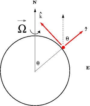
Consider a reference frame fixed to the earth in the Northern Hemisphere at the latitude angle 90 - [math]\theta[/math]. In a standard spherical coordinate system the "z-axis" is directed towards the north pole and [math]\theta[/math] is the polar angle measures from this fixed zenith direction, [math]\phi[/math] is the azimuthal angle corresponding to longitudinal (east-west). Lines of latitude represent the angle measured from the equator to one of the Earth's poles (90 - [math]\theta[/math])

Media:TF_UCM_MiNF_CoriolisRefFrame1.xfig.txt

The non-inertial frame shown above has the [math]\hat x[/math] axis pointing to the west and the [math]\hat y[/math] axis pointing upward along the radial direction from the Earth's center.

The rotation vector [math]\vec \Omega[/math] as described in the non-inertial frame is

[math]\vec \Omega = \cos \theta \hat j + \sin \theta \hat k[/math]

I you launch a projectile in the Northern Hemisphere so its velocity tangential to the Earth's surface and moving from the equator towards the north pole, the projectile will be deflected towards the east (right).

[math] \vec v = v \hat k[/math]

[math]\vec v \times \vec \Omega =\left( \begin{array}{ccc} \hat i & \hat j & \hat k\\ 0 & 0 & v \\0 & \Omega \cos \theta & \Omega \sin \theta \end{array} \right) = - v\Omega \cos \theta \hat i[/math] East

If you launch the projectile towards the equator from the Northern hemisphere.

[math]\vec v \times \vec \Omega =\left( \begin{array}{ccc} \hat i & \hat j & \hat k\\ 0 & 0 & -v \\0 & \Omega \cos \theta & \Omega \sin \theta \end{array} \right) = v\Omega \cos \theta \hat i[/math] West

In both cases the projectile is deflected to the right of its velocity direction.

How about a projectile launched to the West (East)

[math]\vec v \times \vec \Omega =\left( \begin{array}{ccc} \hat i & \hat j & \hat k\\ \pm v & 0 & 0 \\0 & \Omega \cos \theta & \Omega \sin \theta \end{array} \right) = v\Omega \left ( \mp \sin \theta \hat j \pm \cos \theta \hat k \right ) [/math]

A projectile moving West (East) will deflected down(up) and to the right of its trajectory

What happens in the Southern Hemisphere?

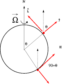
The rotation vector [math]\vec \Omega[/math] as described in the non-inertial frame in the Southern Hemisphere is

[math]\vec \Omega = \cos \theta \hat j + \sin \theta \hat k \;\;\;\;\; \theta \gt 90[/math]

[math] = - \left |\cos \theta \right | \hat j + \sin \theta \hat k [/math]

Now if

Projectile directed from South to North

[math]\vec v \times \vec \Omega = v\Omega \left | \cos \theta \right | \hat i[/math] west

In the Northern hemisphere a projectile would swerve East if you directed it to the North

Projectile directed from South to North

[math]\vec v \times \vec \Omega = - v\Omega \left | \cos \theta \right | \hat i[/math] East

How about a projectile launched to the West (East)

[math]\vec v \times \vec \Omega = v\Omega \left ( \mp \sin \theta \hat j \mp \left | \cos \theta \right |\hat k \right ) [/math]

A projectile moving West (East) in the Souther Hemisphere will deflected down(up) and to the left of its trajectory

Coriolis effect on storm systems

The Earth (and a non-inertial reference frame attached to it) has a rotational velocity

[math]\mathbf \Omega = \frac{ 2 \pi \mbox {radians}}{24 \times 3600 \mbox{seconds}} = 7.3 \times 10^{-5} \frac{\mbox {rad}}{ \mbox{s}}[/math]

Weather systems involve a large mass of air moving at speeds up to 100 miles per hour in the case of a tropical storms.

[math]\Rightarrow a = 2 v \Omega = 2 \times 50 \frac{ \mbox {m}}{\mbox{s}} \times 7.3 \times 10^{-5} \frac{\mbox {rad}}{ \mbox{s}} = 0.007 \frac{ \mbox {m}}{\mbox{s}^2} [/math]

Over large distances this acceleration can have an effect on the course of a storm but not the short distances involved in tornados.

Tropical storms (cyclones) are examples of how the coriolis force determine the rotational direction of an air mass that is quickly moving towards a low pressure area. As the air mass moves along the pressure gradient is is deflected to the right. This results in a clockwise (counter-clockwise) rotation in teh Northern (Southern) hemisphere. The radius of the cyclone can be estimated as

[math]F_{\mbox{Cor}} = m \frac{v^2}{R} = m 2v \Omega \cos \theta \Rightarrow R = \frac{v}{2\Omega \cos \theta}[/math] ( or [math]\sin[/math] of the latitude angle)

[math]R=\frac{v}{2\Omega \cos \theta} = \frac{50 \frac{ \mbox {m}}{\mbox{s}}}{2 \cdot 7.3 \times 10^{-5} \frac{\mbox {rad}}{ \mbox{s}} \cos \theta} = \frac{ 3 \times 10^{5}\mbox {m}}{\cos \theta} =\frac{ 186 \mbox {miles}}{\cos \theta} [/math]

Free fall

Consider an object of mass m close to the surface of the earth and falling in a vacuum.

As viewed from a non-inertial reference frame attached to the rotating earth Newton's second law is

[math] \left ( \sum \vec F \right )_{\mathcal S} = \left ( \sum \vec F \right )_{\mathcal S_0} + \vec F_{\mbox{cor}} + \vec F_{\mbox{cf}} [/math]

The equation of motion may be written as

[math] \vec \ddot r = \vec {g}_0 + 2\vec \dot r \times \vec \mathbf \Omega + \left (\vec \mathbf \Omega \times \vec r\right ) \times \vec \mathbf \Omega [/math]

[math] = \vec {g} + 2\vec \dot r \times \vec \mathbf \Omega [/math]

where

[math]\vec{g}_0 =[/math] the acceleration due to a non-rotating earth

[math]\vec g =\vec {g}_0 + \left (\vec \mathbf \Omega \times \vec r\right ) \times \vec \mathbf \Omega [/math] the acceleration observed

Note

by expressing the equation of motion in terms of \vec g you remove the dependence of [math]\vec r[/math] leaving only a dependence on [math]\vec \dot r[/math] and [math]\vec \ddot r[/math]

If I use a coordinate system where the x-axis if pointing East then the z-axis will be pointing radially upward such that

left

[math]\vec v = \dot x \hat i + \dot y \hat j + \dot z \hat k[/math]

[math]\vec v \times \vec \Omega =\left( \begin{array}{ccc} \hat i & \hat j & \hat k \\ \dot x & \dot y & \dot z \\0 & \Omega \sin \theta & \Omega \cos \theta \end{array} \right) = \Omega \left ( (\dot y \cos \theta - \dot z \sin \theta) \hat i - \dot x \cos \theta \hat j + \dot x \sin \theta \hat k \right ) [/math]

[math] \vec \ddot r = \vec {g} + 2\vec \dot r \times \vec \mathbf \Omega [/math]

[math] = -g \hat k + 2\Omega \left ( (\dot y \cos \theta - \dot z \sin \theta) \hat i - \dot x \cos \theta \hat j + \dot x \sin \theta \hat k \right ) [/math]

[math] = 2\Omega (\dot y \cos \theta - \dot z \sin \theta) \hat i - 2 \Omega \dot x \cos \theta \hat j + (2 \Omega \dot x \sin \theta -g )\hat k [/math]

writing out the individual components

[math]\ddot x =2\Omega (\dot y \cos \theta - \dot z \sin \theta)[/math]

[math]\ddot y =- 2 \Omega \dot x \cos \theta[/math]

[math]\ddot z =2 \Omega \dot x \sin \theta -g[/math]

0th order Approx

let

[math]\Omega \equiv 0[/math]

Then

x-directions

[math]\ddot x = 0[/math]

[math]\int_{\dot x_0}^{\dot x} d\dot x = \int_{t_0}^{t} 0 dt[/math]

[math]\Rightarrow \dot x =\dot x_0[/math] : integrate and the constant is the initial velocity of the projectile

[math] \int_{x_0}^{x} d x = \int_{t_0}^{ t} \dot x_0 dt[/math] : integrate again

[math] \Rightarrow x = \dot x_0 t + x_0[/math] :

similarly in the y-direction

[math]y = \dot y_0 t + y_0[/math]

z-direction

[math]\ddot z = -g[/math]

[math]\int_{\dot z_0}^{\dot z} d\dot z = \int_{t_0}^{t} -g dt[/math]

[math]\Rightarrow \dot z = -gt + \dot z_0[/math]

[math] \int_{z_0}^{z} d z = \int_{t_0}^{ t} (-gt + \dot z_0) dt[/math]

[math] \Rightarrow z = \dot z_0 t + z_0 - \frac{1}{2}gt^2[/math]

1st order Approx

Return to the original system of the equations of motion

[math]\ddot x =2\Omega (\dot y \cos \theta - \dot z \sin \theta)[/math]

[math]\ddot y =- 2 \Omega \dot x \cos \theta[/math]

[math]\ddot z =2 \Omega \dot x \sin \theta -g[/math]

substitute the 0th order solutions and integrate again

x-direction

[math]\ddot x =2\Omega (\dot y \cos \theta - \dot z \sin \theta)[/math]

[math] =2\Omega (\dot y_0 \cos \theta - ( -gt + \dot z_0) \sin \theta)[/math]

[math]\int_{\dot x_0}^{\dot x} d\dot x =\int_{t_0}^{t} \left [ 2\Omega (\dot y_0 \cos \theta - ( -gt + \dot z_0) \sin \theta)\right ] dt[/math]

[math]\Rightarrow \dot x = 2\Omega \left [ \dot y_0 \cos \theta t + \left ( \frac{1}{2} gt^2 - \dot z_0 t \right ) \sin \theta \right ] + \dot x_0[/math]

[math]\int_{\dot x_0}^{\dot x} dx = \int_{t_0}^{t} \left [ 2\Omega \dot y_0 \cos \theta t + 2\Omega \left ( \frac{1}{2} gt^2 - \dot z_0 t \right ) \sin \theta + \dot x_0 \right ] dt[/math]

[math]\Rightarrow x = \Omega \dot y_0 \cos \theta t^2 + \Omega \frac{1}{3} g\sin \theta t^3 - \Omega \dot z_0\sin \theta t^2 + \dot x_0 t[/math]

[math] = \Omega \left ( \dot y_0 \cos \theta - \dot z_0 \sin \theta \right )t^2 + \Omega \frac{1}{3} g\sin \theta t^3 + \dot x_0 t[/math]

y-direction

[math]\ddot y =- 2 \Omega \dot x \cos \theta[/math]

[math] =- 2 \Omega \left ( 2\Omega \dot y_0 \cos \theta t + 2\Omega \left ( \frac{1}{2} gt^2 - \dot z_0 t \right ) \sin \theta + \dot x_0 \right ) \cos \theta[/math]

[math] =- 2 \Omega \dot x_0 \cos \theta[/math] : ignoring [math] \Omega^2[/math] higher order terms

[math]\int_{\dot y_0}^{\dot y} d \dot y =- \int_{t_0}^{t} 2 \Omega \dot x_0 \cos \theta dt[/math]

[math]\Rightarrow \dot y =- 2 \Omega \dot x_0 \cos \theta t + \dot y_0[/math]

[math]\int_{y_0}^{y} d y =- \int_{t_0}^{t} 2 \Omega \dot x_0 \cos \theta t dt + \int_{t_0}^{t} \dot y_0 dt[/math]

[math]\Rightarrow y =- \Omega \dot x_0 \cos \theta t^2 + \dot y_0 t[/math]

z-direction

[math]\ddot z =2 \Omega \dot x \sin \theta -g[/math]

[math]=\ddot 2 \Omega \left ( 2\Omega \dot y_0 \cos \theta t + 2\Omega \left ( \frac{1}{2} gt^2 - \dot z_0 t \right ) \sin \theta + \dot x_0 \right ) \sin \theta -g[/math]

[math]=2 \Omega \dot x_0 \sin \theta -g[/math] : ignoring [math] \Omega^2[/math] higher order terms

[math]\int_{\dot z_0}^{\dot z} d\dot z = \int_{t_0}^{t} \left ( 2 \Omega \dot x_0 \sin \theta -g \right ) dt[/math]

[math]\Rightarrow \dot z = \left ( 2 \Omega \dot x_0 \sin \theta -g \right ) t + \dot z_0[/math] : ignoring [math] :\lt math\gt \int_{z_0}^{z}d z = \int_{t_0}^{t} 2 \left [ \left ( 2 \Omega \dot x_0 \sin \theta -g \right ) t + \dot z_0\right ][/math]

[math]\Rightarrow z = \Omega \dot x_0 \sin \theta t^2 - \frac{1}{2} gt^2 + \dot z_0 t[/math]

General equations of motion

[math]x = \Omega \left ( \dot y_0 \cos \theta - \dot z_0 \sin \theta \right )t^2 + \Omega \frac{1}{3} g\sin \theta t^3 + \dot x_0 t[/math]

[math]y =- \Omega \dot x_0 \cos \theta t^2 + 2 \dot y_0 t[/math]

[math] z = \Omega \dot x_0 \sin \theta t^2 - \frac{1}{2} gt^2 + \dot z_0 t[/math]

If the object is dropped from a height h

[math]\Rightarrow \dot x_0 = \dot y_0 = \dot z_0 = 0[/math]

[math]x = \Omega \frac{1}{3} g\sin \theta t^3 [/math]

[math]y =0[/math]

[math]z = -h = - \frac{1}{2} gt^2 [/math]

[math]\Rightarrow t = \sqrt{\frac{2h}{g}} \;\;\;\;\; x = \Omega \frac{1}{3} g\sin \theta \left ( \frac{2h}{g} \right )^{\frac{3}{2}}[/math]

If I drop an object down an evacuated 100 m deep hole at the equator

[math] x = \Omega \frac{g}{3} \left ( \frac{2h}{g} \right )^{\frac{3}{2}}[/math]

[math] x = (7.3 \times 10^{-5} \frac{1}{\mbox{s}}) \frac{10\mbox{m}}{3\mbox{s}^2} \left ( \frac{200}{10\mbox{s}^2} \right )^{\frac{3}{2}} = 2.2 cm[/math]

Foucault Pendulum

The equation of motion may be written as

[math] \vec \ddot r = \sum \vec F + 2\vec \dot r \times \vec \mathbf \Omega + \left (\vec \mathbf \Omega \times \vec r\right ) \times \vec \mathbf \Omega [/math]

[math] = \vec g_0 + \vec T + 2\vec \dot r \times \vec \mathbf \Omega + \left (\vec \mathbf \Omega \times \vec r\right ) \times \vec \mathbf \Omega [/math]

[math] = \vec {g} + \vec T + 2\vec \dot r \times \vec \mathbf \Omega [/math]

Interpretation of rotating reference frame

Polar

Vector Notation convention:

Position:

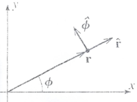
Because [math]\hat{r}[/math] points in a unique direction given by [math]\hat{r} = \frac{\vec{r}}{|r|}[/math] we can write the position vector as

[math]\vec{r} = r \hat{r}[/math]

[math]\vec{r} \ne r \hat{r} +\phi \hat{\phi} [/math]: [math]\phi[/math] does not have the units of length

The unit vectors ([math]\hat{r}[/math] and [math]\hat{\phi}[/math] ) are changing in time. You could express the position vector in terms of the cartesian unit vectors in order to avoid this

[math]\vec{r} = r \cos(\phi) \hat{i} + r \sin(\phi)\hat{j}[/math]

The dependence of position with [math]\phi[/math] can be seen if you look at how the position changes with time.

Velocity in Polar Coordinates

Consider the motion of a particle in a circle. At time [math]t_1[/math] the particle is at [math]\vec{r}(t_1)[/math] and at time [math]t_2[/math] the particle is at [math]\vec{r}(t_2)[/math]

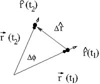
If we take the limit [math]t_2 \rightarrow t_1[/math] ( or [math]\Delta t \rightarrow 0[/math]) then we can write the velocity of this particle traveling in a circle as

[math]\hat{r} (t_2)-\hat{r}(t_1) \equiv \Delta \hat{r} = \Delta \phi \hat{\phi}[/math]

or

[math]\frac{ d \hat{r}}{dt} = \frac{d \phi}{dt} \hat{\phi}[/math]

Thus for circular motion at a constraint radius we get the familiar expression

[math]\vec{v} = \lim_{\Delta t \rightarrow 0} \frac{\vec{r}(t_2)-\vec{r}(t_1)}{\Delta t}= \lim_{\Delta t \rightarrow 0} \frac{r\left( \hat{r}(t_2) - \hat{r}(t_1)\right)}{\Delta t} = r \frac{\Delta \phi}{\Delta t} \hat{\phi} = r \omega \hat{\phi}[/math]

[math]\vec{v} = r \frac{d \phi}{dt} \hat{\phi}[/math]

If the particle is not constrained to circular motion ( i.e.: [math]r[/math] can change with time) then the velocity vector in polar coordinates is

[math]\vec{v}[/math] = [math]\frac{d r}{dt}\hat{r} + r\frac{d \phi}{dt} \hat{\phi}[/math]

or in more compact form

[math]\vec{v}=\vec{\dot{r}} = \dot{r} \hat{r} + r \dot{\phi} \hat{\phi}= v_r \hat{r} + v_{\phi} \hat{\phi}[/math]

linear velocity [math]\equiv v_r [/math] Angular velocity [math]\equiv v_{\phi} [/math]

Finding the derivative directly

Cast the unit vector in terms of cartesian coordinates and take the derivative.

[math]\hat r = \cos \phi \hat{i} + \sin \phi \hat{j}[/math]

[math]\hat \dot{r} = \frac{d \hat{r}}{d \phi} \frac{d \phi}{d t} =\left( \sin \phi \hat{i} - \cos \phi \hat{j} \right ) \dot{\phi}[/math]

[math]= \left ( \hat{\phi} \right ) \dot{\phi} [/math]

Acceleration in Polar Coordinates

Taking the derivative of velocity with time gives the acceleration

[math]\vec{a} = \frac{d \vec{v}}{dt} =\vec{\ddot{r}} [/math]

[math]= \frac{ d \left (\dot{r} \hat{r} + r \dot{\phi} \hat{\phi}= v_r \hat{r} + v_{\phi} \hat{\phi}\right)}{dt}[/math]

[math]= \left ( \frac{ d \dot{r}}{dt} \hat{r} + \dot{r} \frac{ d\hat{r}}{dt} \right) + \left ( \frac{d r}{dt} \dot{\phi} \hat{\phi} +r \frac{d \dot{\phi}}{dt} \hat{\phi} +r \dot{\phi} \frac{d \hat{\phi}}{dt} \right )[/math]

[math]= \left ( \ddot{r} \hat{r} + \dot{r} \dot{\phi}\hat{\phi} \right) + \left ( \dot{r} \dot{\phi} \hat{\phi} +r \ddot{\phi} \hat{\phi} +r \dot{\phi} \frac{d \hat{\phi}}{dt} \right )[/math]

We need to find the derivative of the unit vector [math]\hat{\phi}[/math] with time.

Consider the position change below in terms of only the unit vector [math]\hat{\phi}[/math]

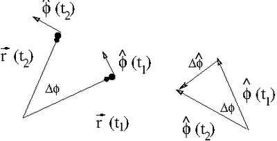
Using the same arguments used to calculate the rate of change in [math]\hat{r}[/math]:

If we take the limit [math]t_2 \rightarrow t_1[/math] ( or [math]\Delta t \rightarrow 0[/math]) then we can write the velocity of this particle traveling in a circle as

[math]\hat{\phi} (t_2)-\hat{\phi}(t_1) \equiv \Delta \hat{\phi} = \Delta \phi (- \hat{r})[/math]

or

[math]\frac{ d \hat{\phi}}{dt} = -\frac{d \phi}{dt} \hat{r}[/math]

[math]\frac{d \hat{\phi}}{dt}= -\dot{\phi} \hat{r}[/math]

Finding the derivative of [math]\hat{\phi}[/math] directly

Cast the unit vector in terms of cartesian coordinates and take the derivative.

[math] \hat{\phi} = \sin \phi \hat{i} - \cos \phi \hat{j} [/math]

[math]\hat \dot{\phi} = \frac{d \hat{\phi}}{d \phi} \frac{d \phi}{d t} =\left( -\cos \phi \hat{i} - \sin \phi \hat{j} \right ) \dot{\phi}[/math]

[math]= \left (- \hat{r} \right ) \dot{\phi} [/math]

Substuting the above into our calculation for acceleration:

[math]\vec{a} = \left ( \ddot{r} \hat{r} + \dot{r} \dot{\phi}\hat{\phi} \right) + \left ( \dot{r} \dot{\phi} \hat{\phi} +r \ddot{\phi} \hat{\phi} +r \dot{\phi} \frac{d \hat{\phi}}{dt} \right )[/math]

[math]= \left ( \ddot{r} \hat{r} + \dot{r} \dot{\phi}\hat{\phi} \right) + \left ( \dot{r} \dot{\phi} \hat{\phi} +r \ddot{\phi} \hat{\phi} +r \dot{\phi} \left( -\dot{\phi} \hat{r}\right) \right )[/math]

[math]= \left ( \ddot{r} -r\dot{\phi}^2 \right) \hat{r} + \left ( 2\dot{r} \dot{\phi} +r \ddot{\phi} \right ) \hat{\phi} [/math]

F_r = m \ddot r \hat r = m \left ( \ddot{r} -r\dot{\phi}^2 \right) \hat{r} =

Forest_Ugrad_ClassicalMechanics