Calculus of Variations

Fermat's Principle

Fermats principle is that light takes a path between two points that requires the least amount of time.

If we let S represent the path of light between two points then

light takes the time [math]t[/math] to travel between two points can be expressed as

The index of refraction is denoted as

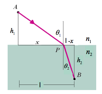
for light traversing an interface with an nindex of refraction $n_1$ on one side and $n_2$ on the other side we would hav e

take derivative of time with respect to [math]x[/math] to find a minimum for the time of flight

or

Generalizing Fermat's principle to determining the shorest path

One can apply Fermat's principle to show that the shortest path between two points is a straight line.

In 2-D one can write the differential path length as

using chain rule

the the path length between two points [math](x_1,y_1)[/math] and [math](x_2,y_2)[/math] is

adding up the minimum of the integrand function is one way to minimize the integral ( or path length)

let

Note: in the above [math]x[/math] is the independent variable in the function while [math]y[/math] and [math]y^{\prime}[/math] depend on [math]x[/math]. The semicolon is used to separate them with the independent variable appearing last

the path integral can now be written in terms of dx such that

To consider deviation away from [math]y(x)[/math] the function [math]\eta(x)[/math] is introduced to denote deviations away from the shortest line and the parameter [math]\alpha[/math] is introduced to weight that deviation

= the difference between the current curve and the shortest path.

let

= A path that is not the shortest path between two points.

Note: It is stipulated that [math]\eta(x)[/math] is independent of [math]\alpha[/math] to ensure that in the [math]\alpha \rightarrow 0[/math] limit, [math]Y(x) = y(x)[/math] and; ie; both the function [math]Y[/math] and its derivative approach [math]y(x)[/math]

let

the deviations in the various paths can be expressed in terms of a differential of the above integral for the path length with respect to the parameter [math]\alpha[/math] as this parameter changes the deviation

The second integral above can by evaluated using integration by parts as

let

:

the difference between the end points should be zero because to keep be sure that the endpoints are the same

The above integral is equivalent to

For the above to be true for any function [math]\eta(x)[/math] then it follows that [math]g(x)[/math] should be zero

= Constant

integrating

http://scipp.ucsc.edu/~haber/ph5B/fermat09.pdf

Euler-Lagrange Equation

The Euler- Lagrange Equation is written as

the above becomes a condition for minimizing the "Action"

Problem 6.16

Brachistochrone problem

Shortest distance betwen two points revisited

Let's consider the problem of determining the shortest distance between two points again.

Previously we determined the shortest distance by assuming only two variables. One was the independent variable [math]x[/math] and the other was dependent on [math]x[/math] ([math] y(x)[/math]).

What happens if the above assumption is relaxed.

To consider all possible paths between two point we should write the path in parameteric form

The functions above are assumed to be continuous and have continuous second derivatives.

Note: the above parameterization includes our previous assumption of the variables if we just let [math]u=x[/math].

Other examples

parabola

circle

ellips

hyperbola

The length of a small segment of the path is given by

now instead of

you have

and the path integral changes from

to

the same arguments are made again

instead of

You now have

instead of

you now have

If you require that the integral not deviate from the shortest path between two points (i.e. it is stationary) Then you are requiring that the integral from path segments that deviate from the shortest path satisfies the equation

and

when

for any function and that vanish at the endpoints and

or

similarly

Apply Euler-Lagrange to shortest path problem revisited

= constant

similarly

Shortest path along a sphere

= constant

Assume the location of the first point is at [math]\theta_1=0[/math] </math>

The curves of constant [math]\phi[/math] are lines of longitude and are great circles which are geodesics (the shortest lines between two points on a shphere)

Brachystochrone problem

In the brachystochrone (Greek for "shortest time") problem we are determining the path of a bead between two points that takes the shortest time when the bead is constrained to slide along a wire without friction and in the presence of gravity.

The fall time for the bead is given by

Using conservation of energy one may cast the beads velocity as

This problem is similar to the shortest distance between two points problem above in that one can write the time variation that you wish to minimize in terms of the path variation

This time however there is an external driving force which is a function of the distance [math]y[/math]. So instead of writing the distance variation [math]ds[/math] as a function of [math]dx[/math] with [math]y(x)[/math] we will want to write it as a function of [math]dy[/math] with [math]x(y)[/math]

then

since[math] f[/math] is an explicit function of [math]y[/math] and

then we can use the Euler-Lagrange equation

Notice how the variables x & y have been interchanged now that [math]x[/math] is written as a function of[math] y (x^{\prime}(y))[/math] whereas before [math]y[/math] was written as a function of [math]x (y^{\prime}(x))[/math]

constant

= constant

or

= constant

using the foresight of working this problem before , the convenient constant is defined as

alternate form of Euler-Lagrange equation

Brachistochrone problem revisited

Consider the Brachistochrone problem again but this time do not cast [math]x^{\prime}[/math] as a function of [math]y[/math]

The fall time for the bead is given by

Using conservation of energy one may cast the beads velocity as

This problem is similar to the shortest distance between two points problem above in that one can write the time variation that you wish to minimize in terms of the path variation

then

BUT the above function appears to be independent of x and

alternate form of Euler-Lagrange's equation (the first integral)

In the previous problems of finding the shortest distance between two point in 2-D and 2 point on the surface of the sphere, the extreme function [math]f[/math] was independent of [math]x[/math] (or [math]\phi[/math])

for the 2-D line

for the geodesic

there are some problems where the functional dependence of [math]f[/math] on [math] x[/math] or [math]\theta[/math] is not explicit

because of this we need to use the chain to take the total derivative of the function [math]f(y,y^{\prime},x)[/math] with respect to [math]x[/math]

Notice

substitution in for[math] y^{\prime\prime}[/math] and moving terms around

rearranging

Euler-Lagrange Equation

Then the alternate form of Euler-Lagrange's equation is

returning to Brachistochrone

Consider the Brachistochrone problem again but this time do not cast [math]x^{\prime}[/math] as a function of [math]y[/math]

The fall time for the bead is given by

Using conservation of energy one may cast the beads velocity as

This problem is similar to the shortest distance between two points problem above in that one can write the time variation that you wish to minimize in terms of the path variation

then

BUT the above function appears to be independent of x and

Using the alternate form of Euler-Lagrange's equation is

constant

let

substituting

to find [math]x[/math] just return to definition of [math]y^{\prime}[/math]

integrating

Soup film (cycloid)

consider the problem of the soap bubble formed between two circular rings. You stack two rings on top of each other in soapy water and then pull them apart after removing them from the water together where a film is created between the rings in a cylindrical shape.

https://www.fields.utoronto.ca/programs/scientific/12-13/Marsden/FieldsSS2-FinalSlidesJuly2012.pdf

Forest_Ugrad_ClassicalMechanics

Forest UCM CoV

Contents

Calculus of Variations

Fermat's Principle

Generalizing Fermat's principle to determining the shorest path

Euler-Lagrange Equation

Shortest distance betwen two points revisited

Apply Euler-Lagrange to shortest path problem revisited

Shortest path along a sphere

Brachystochrone problem

alternate form of Euler-Lagrange equation

Brachistochrone problem revisited

alternate form of Euler-Lagrange's equation (the first integral)

returning to Brachistochrone

Soup film (cycloid)

Navigation menu

Search