|
|
| (9 intermediate revisions by the same user not shown) |
| Line 513: |
Line 513: |
| | :<math>p_2^{\mu} = ( E_2,\vec 0) = (0.000511,0)</math> | | :<math>p_2^{\mu} = ( E_2,\vec 0) = (0.000511,0)</math> |
| | | | |
| − | :v_{cm} = \frac{m_1 p_1}{m_1+m_2} | + | :<math>v_{cm} = \frac{m_1 v_1}{m_1+m_2}</math> |
| | | | |
| | | | |
| Line 527: |
Line 527: |
| | P2.SetPxPyPzE(0,0,0,0.000511) | | P2.SetPxPyPzE(0,0,0,0.000511) |
| | Check that you get the mass of the electron in Units of GeV | | Check that you get the mass of the electron in Units of GeV |
| | + | |
| | + | |
| | + | The invariant mass of the particle is given by |
| | | | |
| | root [36] P1.Mag() | | root [36] P1.Mag() |
| | (const Double_t)5.11000016012715737e-04 | | (const Double_t)5.11000016012715737e-04 |
| | + | |
| | + | The Beta and Gamma of the Particle are Given by |
| | + | |
| | + | |
| | + | P1.Beta() |
| | + | (const Double_t)9.99999998920987565e-01 |
| | + | root [42] P1.Gamma() |
| | + | (const Double_t)2.15264184050203912e+04 |
| | + | |
| | + | |
| | + | The Kinetic Energy (<math>(\gamma-1)m_oc^2</math>) is Given by |
| | + | |
| | + | root [43] (P1.Gamma()-1)*0.511 |
| | + | (const double)1.09994888049654201e+04 |
| | + | root [46] (P1.Gamma()-1)*P1.Mag() |
| | + | (const double)1.09994891496458251e+01 |
| | | | |
| | | | |
| Line 536: |
Line 555: |
| | Construct the boost vector | | Construct the boost vector |
| | | | |
| − | TVector3 Vcm; | + | |
| | + | TLorentzVector CMS; |
| | + | |
| | + | CMS=P1+P2; |
| | | | |
| − | Vcm.SetX(P1.Px()/(P1.E()+P2.E())) | + | P1.Boost(-CMS.BoostVector()); |
| − | Vcm.SetY(P1.Py()/(P1.E()+P2.E())) | + | P2.Boost(-CMS.BoostVector()); |
| − | Vcm.SetZ(P1.Pz()/(P1.E()+P2.E())) | + | |
| − | Vcm.Mag() | + | root [138] P1.Px() |
| − | (const Double_t)9.99999998920987565e-01 | + | (const Double_t)5.30129176950140391e-02 |
| | + | root [139] P2.Px() |
| | + | (const Double_t)(-5.30129176949399178e-02) |
| | + | |
| | + | A final state moller scattering event from GEANT4 has |
| | + | |
| | + | The scattered electron |
| | | | |
| − | P1.Boost(Vcm) | + | P3.SetPxPyPzE(0.433025,-0.858867,10999.6,sqrt(0.433025*0.433025+0.858867*0.858867+10999.6*10999.6+ 0.000511*0.000511)) |
| | | | |
| − | P1.Px()
| + | The moller electron |
| − | (const Double_t)4.73581204910448636e+05
| |
| | | | |
| − |
| + | P4.SetPxPyPzE(-0.433025,0.858867,0.905366,sqrt(0.433025*0.433025+0.858867*0.858867+0.905366*0.905366+ 0.000511*0.000511)) |
| − | P2.Boost(Vcm) | |
| − | P2.Px()
| |
| − | (const Double_t)1.09999997930962827e+01
| |
| | | | |
| | | | |
| | + | <pre> |
| | + | CMS=P3+P4 |
| | | | |
| | | | |
| | + | P3.Boost(-CMS.BoostVector()); |
| | + | root [191] P4.Boost(-CMS.BoostVector()); |
| | + | root [192] P3.Px() |
| | + | (const Double_t)4.33024999999999993e-01 |
| | + | root [193] P4.Px() |
| | + | (const Double_t)(-4.33024999999999993e-01) |
| | + | root [194] P3.Py() |
| | + | (const Double_t)(-8.58867000000000047e-01) |
| | + | root [195] P4.Py() |
| | + | (const Double_t)8.58867000000000047e-01 |
| | + | root [196] P3.Pz() |
| | + | (const Double_t)4.78021531980484724e+01 |
| | + | root [197] P4.Pz() |
| | + | (const Double_t)(-4.78021531981362244e+01) |
| | + | root [198] P3.E() |
| | + | (const Double_t)4.78118292245973180e+01 |
| | + | root [199] P4.E() |
| | + | (const Double_t)4.78118292247171723e+01 |
| | | | |
| | + | </pre> |
| | | | |
| | | | |
| | [http://iac.isu.edu/mediawiki/index.php/Classes Back to Classes] | | [http://iac.isu.edu/mediawiki/index.php/Classes Back to Classes] |
Lorentz Transformations
The picture below represents the relative orientation of two different coordinate systems [math](S, S^{\prime})[/math] . [math]S[/math] is at rest (Lab Frame) and [math]S^{\prime}[/math] is moving at a velocity v to the right with respect to frame [math]S[/math].
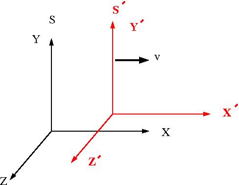
The relationship between the coordinate[math] (x,y,z,ct)[/math] of an object in frame [math]S[/math] to the same object described using the coordinates [math](x^{\prime},y^{\prime},z^{\prime},ct^{\prime})[/math] in frame [math]S^{\prime}[/math] is geven by the Lorentz transformation:
Notation
The relativistic transformation used to transform the coordinates of an object observed in the rest frame [math]S[/math] to a moving reference frame[math] S^{\prime}[/math] is given by:
- [math]x^{\mu^{\prime}} = \sum_{\nu=0}^3 \Lambda_{\nu}^{\mu} x^{\nu}[/math]
where
- [math] x^0 \equiv ct[/math]
- [math]x^1 \equiv x[/math]
- [math]x^2\equiv y[/math]
- [math]x^3\equiv z[/math]
- [math]\Lambda = \left [ \begin{matrix} \gamma & -\gamma \beta & 0 & 0 \\ -\gamma \beta & \gamma &0 &0 \\ 0 &0 &1 &0 \\ 0 &0 &0 &1\end{matrix} \right ][/math]
- [math]\beta = \frac{v}{c} = \frac{pc}{E}[/math]
- [math]\gamma = \frac{1}{\sqrt{1 -\beta^2}} = \frac{E_{tot}}{mc^2}[/math]
- NOTE
- It is common in particle physics to define [math] c \equiv 1[/math] making [math]\gamma = \frac{E}{m}[/math] where [math]m[/math] is in units of [math]\frac{\mbox{MeV}}{\mbox{c}^2}[/math]
- example
- [math]x^{0^{\prime}} = \sum_{\nu=0}^2 \Lambda_{\nu}^0 x^{\nu} = \Lambda_0^0 x^0 + \Lambda_1^0 x^1 \Lambda_2^0 x^2 + \Lambda_3^0 x^2[/math]
- [math]ct^{\prime}= \gamma x^0 - \gamma \beta x^1 + 0 x^2 + 0 x^3 = \gamma ct - \gamma \beta x = \gamma(ct -\beta x)[/math]
- Or in matrix form the tranformation looks like
- [math]\left ( \begin{matrix} ct^{\prime} \\ x^{\prime} \\ y^{\prime} \\ z^{\prime} \end{matrix} \right )= \left [ \begin{matrix} \gamma & -\gamma \beta & 0 & 0 \\ -\gamma \beta & \gamma &0 &0 \\ 0 &0 &1 &0 \\ 0 &0 &0 &1\end{matrix} \right ] \left ( \begin{matrix} ct \\ x \\ y \\ z \end{matrix} \right )[/math]
- Note
- Einstein's summation convention drops the [math]\sum[/math] symbols and assumes it to exist whenever there is a repeated subscript and uperscript
- ie; [math]x^{\mu^{\prime}} = \Lambda_{\nu}^{\mu} x^{\nu}[/math]
- in the example above the[math] \nu[/math] symbol is repeated thereby indicating a summation over [math]\nu[/math].
Momentum 4-vector
The momentum 4 -vector is denoted as:
- [math]p^{\mu} \equiv (\frac{E}{c} , \vec{p})[/math]
- [math]p_{\mu} \equiv (\frac{E}{c} , -\vec{p})[/math]
- [math]p_{\mu}p^{\mu} = \frac{E^2}{c^2} - p^2 \equiv E^2 - p^2 = m^2[/math]
- Note
- There is another convention used for 4-vector notation by Perkins and Koller which goes like this
- [math]p^{\mu} \equiv (\vec{p},iE)[/math]
- [math]p_{\mu} \equiv (\vec{p},iE)[/math]
Trig Method
Another way to represent the Lorentz transformation is by using the substitution
- [math]\sin (\alpha) \equiv \beta \equiv \frac{v}{c}[/math]
- [math]\cos(\alpha) \equiv \frac{1}{\gamma} \equiv \sqrt{1 - \beta^2}[/math]
- The Matrix form of the tranformation looks like
- [math]\left ( \begin{matrix} ct^{\prime} \\ x^{\prime} \\ y^{\prime} \\ z^{\prime} \end{matrix} \right )= \left [ \begin{matrix} \sec(\alpha) & -\tan(\alpha) & 0 & 0 \\ -\tan(\alpha) & \sec(\alpha) &0 &0 \\ 0 &0 &1 &0 \\ 0 &0 &0 &1\end{matrix} \right ] \left ( \begin{matrix} ct \\ x \\ y \\ z \end{matrix} \right )[/math]
- Or the reverse transformation
- [math]\left ( \begin{matrix} ct \\ x \\ y \\ z \end{matrix}\right )= \left [ \begin{matrix} \sec(\alpha) & \tan(\alpha) & 0 & 0 \\ \tan(\alpha) & \sec(\alpha) &0 &0 \\ 0 &0 &1 &0 \\ 0 &0 &0 &1\end{matrix} \right ] \left ( \begin{matrix} ct^{\prime} \\ x^{\prime} \\ y^{\prime} \\ z^{\prime} \end{matrix} \right )[/math]
- Notice that you just needed to change the signs for the inverse matrix [math]\Lambda^{-1}[/math]
Proper Time and Length
Proper Time
- Proper Time [math]\Tau[/math]
- The time measured in the rest frame of the clock. The time interval is measured at the same x,y,z coordinates because the clock chose is in a frame which is not moving (rest frame).
The time given in any frame (t) = [math]\gamma \Tau[/math]
- Note
- since [math]\gamma \gt 1[/math] you expect the Proper time interval to be the smallest
Proper Length
- Proper Length[math] (c\Tau)[/math]
- The length of an object in the object's rest frame.
Invariant Length
Transformation Examples
Decay of a Particle at Rest to 2 Bodies
Consider the decay of the [math]\rho_0[/math] meson of mass [math]M[/math] at rest into two pions ([math]\pi^+[/math] and [math]\pi^-[/math] ) of mass [math]m_1[/math] and [math]m_2[/math] respectively.
File:NeutralRhoMesonDecayDiagram.jpg
The diagram above shows a [math]\rho_0[/math] meson at rest in the lab which then decays into two pions of momentum [math]p_1[/math] and [math]p_2[/math] in the center of momentum frame of the [math]\rho_0[/math] meson.
Our goal is to determine the momentum and energy of each pion ([math]E_1[/math] & [math]E_2[/math]) resulting from the decay of the Mother particle.
Conservation of 4-Momentum implies that if [math]P^{\mu}[/math] represents the total momentum of the system before the decay then
- [math]P^{\mu} = (E,0) =(M,0) = \left ( p_1 \right )^{\mu} + \left ( p_2 \right)^{\mu}[/math]
- [math]\Rightarrow 0 = \vec{p}_1 + \vec{p}_2[/math]
or
- [math]\vec{p}_1 = - \vec{p}_2[/math]
Let
- [math]p \equiv |\vec{p}_1 | = |\vec{p}_2 |[/math]
Conservation of Energy
- [math]\Rightarrow E_{tot} = M = E_1 + E_2 = \sqrt{m_1^2 + p^2} + \sqrt{m_2^2 + p^2}[/math]
solving for p
- [math]\Rightarrow p = \frac{1}{2M} \sqrt{[M^2 - (m_1-m_2)^2][M^2-(m_1+m_2)^2]}[/math]
- [math]\Rightarrow M \ge m_1 + m_2[/math] is required to avoid the unphysical condition that the momentum of the particles after a decay would be an imaginary number
Using
- [math]p \equiv |\vec{p}_1 | = |\vec{p}_2 |[/math]
- [math]E_1^2 - m_1^2 = E_2^2 - m_2^2[/math]
- [math]\Rightarrow E_2 = \sqrt{E_1^2 - m_1^2 + m_2^2}[/math]
Combine this with the conservation of energy equation above:
- [math] E_1 + E_2 = E_1 + \sqrt{E_1^2 - m_1^2 + m_2^2} = M[/math]
- [math]\Rightarrow E_1 - M = \sqrt{E_1^2 - m_1^2 + m_2^2}[/math]
Square both sides of the above equation
- [math]E_1^2 -2ME_1 + M^2 = E_1^2- m_1^2 + m_2^2[/math]
- [math]\Rightarrow E_1 = \frac{M^2+m_1^2-m_2^2}{2M}[/math]
Similarly
- [math] E_2 = \frac{M^2+m_2^2-m^2_1}{2M}[/math]
- Note
- [math]\vec{p}_1 = -\vec{p}_2[/math]
- [math]\Rightarrow[/math] The daughter particles (pions) from the decay of the Mother particle [math](\rho)[/math] travel in opposite directions with respect to eachother ( ie; they are "back - to -back")
- This means that there is no preferential direction for the decay (the particles are distributed isotropically such that they are back-to-back)
Decay of Moving Particle to 2 Bodies (decay in flight)
- [math]P^{\mu} = (E,\vec{p}_{tot}) =(M,\vec{p}_{tot}) = \left ( p_1 \right )^{\mu} + \left ( p_2 \right)^{\mu}[/math]
Assuming that the Mother particle is moving along the Z-axis, then the momentum of the daughter particles perpendicular to the Z-axis (transverse components:[math]\vec{p}_{1,\perp}[/math] and [math]\vec{p}_{2,\perp}[/math]) are equal and opposite by conservation of momentum.
- [math]\vec{p}_{1,\perp}\equiv -\vec{p}_{2,\perp}[/math]
The center of momentum frame is moving such that
- [math]\beta_{CM} = \frac{p_{tot}}{M}[/math]
- [math]\gamma_{CM} = \frac{E_{tot}}{M}[/math]
A Lorentz transformation of the kinematics for particle 1 between the Center of Momentum (cm) frame and the lab is given by:
- [math]E_1 = \gamma_{cm}(E_1^{CM} + \beta_{cm}p_{1,z}^{CM})[/math]
- [math]p_{1,z} = \gamma_{CM}(p_{1,z}^{CM} + \beta_{cm} E_1^{CM})[/math]
- [math]p_{1,\perp} = p_{\perp}^{CM}[/math]
where
- [math]E_1^{CM}[/math] = Kinetic Energy (not total) of particle 1 in the center of momentum (CM) reference frame
- [math]p_{1,z}^{CM}[/math] = momentum of particle 1 along the direction of the mother particle in the CM frame
- [math]p_{1,\perp}[/math] = the component of particle 1's momentum perpendicular to Mother particle's momentum
- You can now use the results for [math]E_1[/math] and [math]p_1=p[/math] from the previous section where the Mother particle is at rest to determine the kinematics of the particles in the lab frame given that you know the initial 4-Momentum of the mother particle. You will need to specify the daugher decay angles in the CM frame in order to find the momentum components [math]p_z[/math] and [math]p_{\perp}[/math].
- It can be shown that the lab angle for daughter particle 1 ([math]\theta_1[/math]) is given by
- [math]\tan(\theta_1) = \frac{\sin(\theta_1^{CM})}{\gamma_{CM}\left (\frac{\beta_{CM}}{\beta_1^{CM}} + \cos(\theta_1^{CM}) \right )}[/math]
where
- [math]\beta_1^{CM} = \frac{p_1}{E} = \beta[/math] for daughter particle 1 in CM frame.
One could also find [math]\vec{p}_1[/math] without using the Lorentz transformation. Just use conservation of Energy and Momentum:
- [math]E_{tot} = E_1^{tot} + E_2^{tot} = \sqrt{m_1^2 + p_1^2} + \sqrt{m_2^2 + p_2^2}[/math]
- [math]\vec{p_{tot}} = \vec{p}_1 + \vec{p}_2[/math]
Solve the conservation of momentum equation for [math]p_2^2[/math]
- [math]p_2^2 = (\vec{p_{tot}}- \vec{p}_1)^2
[/math]
and substitute the above for [math]p_2^2[/math] in the Conservation of Energy equation above. The dot product gives you the angle between the daughter momentum and the Mother momentum ([math]\theta_1[/math]) as a variable. After a lot of algebra you can show that
- [math]p_1 = \frac{\left ( M^2 + m_1^2 -m_2^2 \right ) p_{tot} \cos(\theta_1) \pm 2E\sqrt{M^2p^2 - m_1^2p^2_{tot} \sin^2(\theta_1)}}{2 \left( M^2 + p^2 \sin^2(\theta_1)\right )}[/math]
- Note
- [math]p[/math] is the momentum of the two daughter particles in the CM frame which was derived when the Mother particle was at rest. [math]p_{tot}[/math] is the momentum of the Mother particle.
In order for a real solution
- [math]M^2p^2 - m_1^2p^2_{tot} \sin^2(\theta_1) \ge 0[/math]
- [math]\Rightarrow \frac{M p}{m_1 p_{tot}} \ge \sin(\theta_1)[/math]
If [math]\frac{M p}{m_1 p_{tot}} \gt 1[/math] then [math]\theta_1[/math] can be any angle and the "-" sign possibility in "[math]\pm[/math]" is rejected to avoided negative values for [math]p_1[/math] when [math]\theta_1[/math] > [math]\frac{\pi}{2}[/math].
If [math]\frac{M p}{m_1 p_{tot}} \lt 1[/math] then the maximum emmission angle for daughter 1 is given by
- [math]\sin(\theta_1^{max}) = \frac{M p}{m_1 p_{tot}}[/math]
The "[math]\pm[/math]" is kept because for each [math]\theta_1 \lt \theta_1^{max}[/math] there are two possible trajectories for daughter particle 1 and as a result 2 trajectories for daughter particle 2.
Decay of Particle to 3 Bodies (Dalitz plot)
Now lets consider the case where a Mother particle of mass [math]M[/math] decays into 3 daughter particles of masses [math]m_1[/math], [math]m_2[/math], and [math]m_3[/math]. The 4-mometum conservation is written as
- [math]P^{\mu} = \left ( p_1 \right )^{\mu} +\left ( p_2 \right )^{\mu} +\left ( p_3 \right )^{\mu}[/math]
The following invariants are defined
- [math]s = P_{\mu}P^{\mu} = M^2[/math]
- [math]s_1 = \left (P -p_1 \right)_{\mu}\left (P -p_1 \right)^{\mu}=\left (p_2 + p_3 \right)_{\mu}\left (p_2 + p_3 \right)^{\mu}[/math]
- [math]s_2 = \left (P -p_2 \right)_{\mu}\left (P -p_2 \right)^{\mu}=\left (p_3 + p_1 \right)_{\mu}\left (p_3 + p_1 \right)^{\mu}[/math]
- [math]s_3 = \left (P -p_3 \right)_{\mu}\left (P -p_3 \right)^{\mu}=\left (p_1 + p_2 \right)_{\mu}\left (p_1 + p_2 \right)^{\mu}[/math]
The invariants [math]s_1[/math], [math]s_2[/math] and [math]s_3[/math] are not independent (the motivation for what is known as a Dalitz plot). Based on the definitions of these invariants and 4-momentum conversation one can show that
- [math]s_1 + s_2 + s_3 = (P^2 -2Pp_1 +p_1^2) +(P^2 -2Pp_2 +p_2^2) + (P^2 -2Pp_3 +p_3^2)[/math]
- [math]=3P^2 -2P(p_1+p_2+p_3) +p_1^2+p_2^2+p_3^2[/math]
- [math]=3P^2 -2P^2 +p_1^2+p_2^2+p_3^2[/math]
- [math]=P^2 +p_1^2+p_2^2+p_3^2[/math]
- [math]=M^2 + m_1^2 + m_2^2 +m_3^2[/math]
- Also Note
- [math]\sqrt{s_1}[/math] is the invariant mass of a subsystem defined by treating daughter particles 2 and 3 as one object. similar interpretations for [math]\sqrt{s_2}[/math] and [math]\sqrt{s_3}[/math].
There are limits to the values of the invariant masses [math]s_1[/math] - [math]s_3[/math]
In the Center of Momentum system we have the
- [math]s_1 = M^2 +m_1^2 - 2ME_1[/math]
because
- [math]E_1 = m_1^2 + p_1^2[/math] we expect [math]E_1 \ge m_1[/math]
This lead to
- [math]\left . s_1 \right |_{max} = M^2 +m_1^2 - 2M(m_1) = (M-m_1)^2[/math]
TO find the minimum value of [math]s_1[/math] we evaluate [math]s_1[/math] in the rest frame of the [math]m_2[/math], [math]m_3[/math] subsystem.
- [math]s_1 = \left (p_2 + p_3 \right)_{\mu}\left (p_2 + p_3 \right)^{\mu}= (E_2^{cm2-3} +E_3^{cm2-3})^2 \gt (m_2 + m_3)^2[/math] : In the CM frame [math]E = \sqrt{p^2 +m^2} = m[/math]
so the limits of s_1 are
- [math](m_2 + m_3)^2 \le s_1 \le (M-m_1)^2[/math]
Invariant mass Dalitz plot Limits
Analagously you can show the the Min - Max limits for the [math]s_1[/math], [math]s_2[/math], and [math]s_3[/math] invariant masses are given by.
- [math](m_3 + m_1)^2 \le s_2 \le (M-m_2)^2[/math]
- [math](m_1 + m_2)^2 \le s_3 \le (M-m_3)^2[/math]
set theory notation is often used to express the above limits as
- [math]s_1 \in \left [ (m_2 + m_3)^2 , (M-m_1)^2 \right ][/math]
- [math]s_2 \in \left [ (m_3 + m_1)^2 , (M-m_2)^2 \right ][/math]
- [math]s_2 \in \left [ (m_1 + m_2)^2, (M-m_3)^2 \right ][/math]
Dalitz plot boundary curve equation
Suppose we wish to plot a curve which describes the depence of s_1 on s_2 (determine s_2 as a function of s_1). This is refered to as a Dalitz plot in which [math]s_2[/math] appears on the x-axis (abscissa) and [math]s_1[/math] appears on the y-axis (ordinate). Becuase of the "squares" in the invariant mass, we can have two values of [math]s_2[/math] for a given value of [math]s_1[/math].
since
- [math]s_2 = \left (p_3 + p_1 \right)_{\mu}\left (p_3 + p_1 \right)^{\mu}[/math]
We should look seek equations for [math]p_1[/math] and [math]p_3[/math] in terms of masses[math](M,m_1,m_2,m_3)[/math] and invariants [math](s,s_1)[/math].
In order to find such expressions lets consider the problem as viewed by a reference frame in which [math]\vec{p}_3[/math] = -[math]\vec{p}_2[/math]. This reference frame is sometimes referred to as the Jackson Frame (JF).
In the JF frame
- [math]\vec{P}^{JF} = \vec{p}_1^{JF}[/math] : because the other two particles cancel the total momentum of the system is carried by [math]m_1[/math].
- [math]s_1 \equiv = \left (P -p_1 \right)_{\mu}\left (P -p_1 \right)^{\mu}[/math]
- [math]=\left [ (E,-\vec{P}) - (E_1,-\vec{p_1})\right ]\left [ (E,\vec{P}) - (E_1,\vec{p}_1)\right ][/math]
- [math]=\left [ (E^{JF},-\vec{P}^{JF}) - (E_1^{JF},-\vec{p}_1^{JF})\right ]\left [ (E^{JF},\vec{P}^{JF}) - (E_1^{JF},\vec{p}_1^{JF})\right ][/math]
- [math]= (E^{JF}-E_1^{JF})^2 : \vec{P}^{JF}=\vec{p}_1^{JF}[/math]
- =[math]\left( \sqrt{M^2+(P^{JF})^2} - \sqrt{m^2+(p_1^{JF})^2}\right)[/math] : Def of [math]E_{tot}[/math]
- =[math]\left( \sqrt{M^2+(p_1^{JF})^2} - \sqrt{m^2+(p_1^{JF})^2}\right)[/math]
where
- [math]E^{JF}[/math] = total energy of Mother particle before it decays
- [math]E_1^{JF}[/math] = total energy of [math]m_1[/math] particle
solving for [math]p_1^{JF}[/math]
- [math]\left( p_1^{JF}\right )^2 = \frac{1}{4s_1} \left [ s_1 -(M-m_1)^2\right ]\left [ s_1 -(M+m_1)^2\right ][/math]
The function [math]\lambda[/math] is defined such that
- [math]\lambda(A,B^2,C^2) = \left [ A -(B-C)^2\right ]\left [ A -(B+C)^2\right ][/math] : notice the "squared" arguments
- [math]=A^2 + B^2 + C^2 -2AB -2BC -2CA
[/math]
since this solution above is so common in relativistic kinematics
- [math]\Rightarrow \left( p_1^{JF}\right )^2 = \frac{1}{4s_1}\lambda(s_1,M^2,m_1^2)
[/math]
Doing an analogous calculation for the other form os s_1
- [math]s_1 =\left (p_2 + p_3 \right)_{\mu}\left (p_2 + p_3 \right)^{\mu}[/math]
we will find
- [math]p_2^{JF} = p_3^{JF} = \frac{1}{4s_1}\lambda(s_1,m^2,m_3^2)[/math]
Lets substitute [math]p_1[/math] and [math]p_3[/math] into the definition for [math]s_2[/math] in the Jackson Frame.
- [math]s_2 = \left (p_3 + p_1 \right)_{\mu}\left (p_3 + p_1 \right)^{\mu}[/math]
- [math]=\left (p_3^{JF} + p_1^{JF} \right)_{\mu}\left (p_3^{JF} + p_1^{JF} \right)^{\mu}[/math]
- [math]=\left [ (E_1^{JF},-\vec{p}_1^{JF}) + (E_3^{JF},-\vec{p}_3^{JF})\right]\left [ (E_1^{JF},\vec{p}_1^{JF}) + (E_3^{JF},\vec{p}_3^{JF})\right][/math]
- [math]= m_1^2 +m_3^2 + 2\left ( E_1^{JF} E_3^{JF} - p_1^{JF} p_2^{JF} \cos(\theta_{13})\right )[/math]
where
- [math]\cos(\theta_{13})[/math] = angle between [math]\vec{p}_1^{JF}[/math] and [math]\vec{p}_3^{JF}[/math]
[math]p_1^{JF}[/math] and [math]p_2^{JF}[/math] are given above we just need to figure out what [math]E_1^{JF}[/math] and [math]E_2^{JF}[/math] are
If we assume [math]s_1[/math] is fixed (you generate the Dalitz plot boundary by determining the two values of [math]s_2[/math] for a given value of [math]s_1[/math]) then
- [math]E_1^{JF} = \frac{1}{2\sqrt{s_1}} (M^2 - s_1 -m_1^2)[/math]
- [math]E_3^{JF} = \frac{1}{2\sqrt{s_1}} (s_1 + m_3^2 -m_2^2)
[/math]
The only remaining unkown is the angle [math](\alpha)[/math] between math>\vec{p}_1^{JF}</math> and [math]\vec{p}_3^{JF}[/math] which we can treat as either [math]\pi[/math] or 0 to determine the min and max values of s_2 for a given value of 2_1.
- [math]s_2= m_1^2 +m_3^2 + 2\left ( E_1^{JF} E_3^{JF} - p_1^{JF} p_2^{JF} \cos(\theta_{13})\right )[/math]
- [math]= m_1^2 +m_3^2 + 2\left ( E_1^{JF} E_3^{JF} \pm p_1^{JF} p_2^{JF} \right )[/math]
- [math]= m_1^2 +m_3^2 + 2\left ( \frac{1}{2\sqrt{s_1}} (M^2 - s_1 -m_1^2) \frac{1}{2\sqrt{s_1}} (s_1 + m_3^2 -m_2^2) \pm p_1^{JF} p_2^{JF} \right )[/math]
Substituting for [math]p_1^{JF}[/math] and [math]p_2^{JF}[/math]
- [math]s_2=m_1^2 +m_3^2 + \frac{1}{s_1} \left ((M^2 - s_1 -m_1^2)(s_1 + m_3^2 -m_2^2) \pm \sqrt{\lambda(s_1,M^2,m_1^2) \lambda(s_1,m_2^2,m_3^2)}\right )[/math]
The above equation for [math]s_2[/math] defines a boundary line of the Dalitz plot. The kinematics of the particles in constrained to the interior of this bounding.
Example:[math] D_s^+[/math] Meson decay
Consider the [math]D_s^+[/math] meson which decays [math]\sim[/math] 5\% of the time into three particles; [math]K^+K^-\pi^+[/math]
- [math]M =1969 MeV[/math] for a[math] D_s^+[/math] Meson
- [math]m_1 = 494 MeV[/math] for a [math] K^+[/math]
- [math] m_2 = 140 MeV[/math] is a [math]\pi^+[/math]
- [math] m_3=494 MeV[/math] is a [math]K^-[/math]
Dalitz Plot limits are:
- X-axis[math] (s_2)[/math]
- Min = [math](m_3 + m_1)^2 = (988 MeV)^2 \; \sim 1 GeV^2[/math]
- Max = [math](M-m_2)^2 = (1829 MeV)^2 = 3.35 GeV^2[/math]
- Y-axis [math](s_1)[/math]
- Min [math](m_2+m_3)^2 \; \sim (634 MeV)^2 = 0.402 GeV^2[/math]
- Max= [math](M-m_1)^2 = (1475 MeV)^2 = 2.2 GeV^2[/math]
The image below is from experiment E698
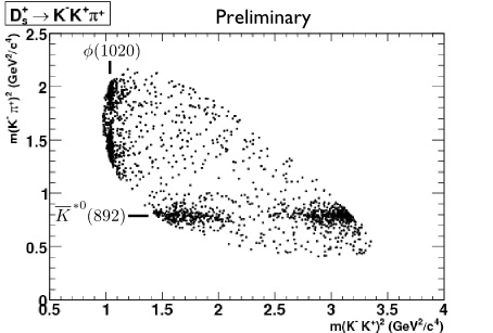
Notice the dark bands which have been labeled [math]\phi(1020)[/math] and [math]\bar{K}^{*0}(892)[/math]. These dark bands indicate a tendency for the decay to clump into states with specific masses, namely [math]s_2=1.04 GeV^2 (\Rightarrow m=1020 MeV)[/math] and [math]s_1=0.796 GeV^2 (\Rightarrow m= 892 MeV^2)[/math]. The isobar model suggests that the [math]D_s^+[/math] decays into two particles and then a third particle. In one case the decay is
- [math]D_s^+ \rightarrow \phi^0 + \pi^+[/math]
and then the [math]\phi[/math] decays via
- [math]\phi^0 \rightarrow K^+ + K^-[/math]
Notice that the dark bands are not infinitely thin but have widths as well. The uncertainty principle ([math]\Delta E \Delta t \gt \hbar[/math]) suggest that only a particle with an infinite lifetime can have a finite , well defined, mass. The width of these dark bands can be used to determine the lifetimes of the intermediate [math]\phi[/math] and [math]\bar{K}^{*0}[/math] states.
Also notice that there are 2 "clumps" of darks spots in each dark band. The limits for [math]s_2[/math] where based on Min/Max values of the [math]\cos(\theta_{13})[/math] term. This term tells us how aligned or misaligned the momentum vecors of [math]m_1[/math] and [math]m_3[/math] (the Kaons)are.
Elastic Scattering
File:ForestRelativity ElasticScateringDiagram.jpg
Given the elastic scattering of 2 particles such that the following properties are
- Known
- [math]m_1[/math] = mass of the incident particle #1
- [math]m_2[/math] = mass of the target particle (at rest) #2
- [math]p_1[/math] = momentum of the incident particle #1
- [math]\theta_1[/math] = scattering angle of particle #1
You can show that
- [math]p_1^{\prime} = \frac{-B \pm \sqrt{B^2 -4AC}}{2A}[/math] = Final momentum of scattered particle #1
- [math]p_2^{\prime} = \left ( p_1^{\prime} \right )^2 -2p_1p_1^{\prime}\cos(\theta_1) + p_1^2[/math] = Final momentum of the target particle
- [math]\sin (\theta_2) = - \frac{p_1^{\prime} \sin(\theta_1)}{p_2^{\prime}}[/math]
where
- [math]A = \left ( \sqrt{p_1^2 +m_1^2} +m_2 \right )^2 -p_1^2 \cos^2(\theta_1)[/math]
- [math]B = -2p_1 \cos(\theta_1) \left ( m_1^2 + m_2 \sqrt{p_1^2 + m_1^2}\right )[/math]
- [math]C = - \left [ m_1^4 + (m_2^2 -m_1^2)(p_1^2 + m_1^2) -m_1^2m_2^2\right ][/math]
In-Elastic Scattering
File:ForestRelativity InelasticScatDiagram.jpg
- List of 4-vectors
- [math]q^{\mu} \equiv ( \omega , \vec{q} )[/math] = momentum transfered from incident particle to target
- [math]k_i^{\mu} \equiv (E_i, \vec{k}_i )[/math] = initial momentum of incident particle
- [math]k_f^{\mu} \equiv (E_f, \vec{k}_f )[/math] = final momentum of incident particle
- [math]q^{\mu} \equiv k_i^{\mu} - k_f^{\mu}[/math] = definition of momentum transfer based on conservation of momentum
Momentum Transfer Squared [math](Q^2)[/math]
The momentum transfer squared is given by
- [math]q_{\mu}q^{\mu} = (E_i - E_f)^2 -(\vec{k}_i - \vec{k}_f ) (\vec{k}_i - \vec{k}_f )[/math]
- [math]=(E_i^2 -2E_iE_f +F_f^2) - ( |\vec{k}_i |^2 - 2 |\vec{k}_i| |\vec{k}_f| \cos(\theta) + | k_f |^2)[/math]
- [math]E^2 = | \vec{k} |^2 +m^2 [/math]
- [math]\Rightarrow q_{\mu}q^{\mu} = \left ( | \vec{k}_i |^2 +m_i^2 - 2 E_i E_f +| \vec{k}_f |^2 +m_f^2\right ) - | \vec{k}_i |^2 - | \vec{k}_f |^2 + 2 | \vec{k}_i | | \vec{k}_f |^2 \cos(\theta)[/math]
- [math]= m_i^2 + m_f^2 - 2 E_i E_f + 2| \vec{k}_i | | \vec{k}_f |^2 \cos(\theta)
[/math]
In the case of electron scattering
- [math]m_i = m_f[/math]
- [math]E_i \sim | \vec{k}_i |[/math]
- [math]E_f \sim | \vec{k}_f |[/math]
- [math]m \ll E[/math]
- [math]\Rightarrow q^2 = -2 | \vec{k}_i | | \vec{k}_f | \left ( 1 - \cos (\theta) \right )[/math]
- [math]= -4 | \vec{k}_i | | \vec{k}_f | \sin^2(\frac{\theta}{2}) \equiv -4 E_i E_f \sin^2(\frac{\theta}{2})[/math]
if[math] q^2 \lt 0 \Rightarrow[/math] spacelike (scattering)
if [math]q^2 \gt 0 \Rightarrow[/math] timelike (free particle)
The Momentum Transfer squared for scattering is define as [math]Q^2[/math] such that
- [math]Q^2 = -q^2[/math]
Missing Mass [math](W)[/math]
Consider an inelastic scattering process where the particles have the 4-Momentum vectors defined as
- [math]\left ( p_e^{\mu} \right ) \equiv (E_i, \vec{k}_i)[/math] = initial momentum 4-vector of the incident electron
- [math]\left ( p_p^{\mu} \right ) \equiv (M_p, 0)[/math] = initial momentum 4-vector of the target proton
- [math]\left ( p_e^{\mu} \right )^{\prime} \equiv (E_f, \vec{k}_f)[/math] = final momentum 4-vector of the scattered electron
- [math]\left ( p_p^{\mu} \right )^{\prime} \equiv (E_X, \vec{p}_X)[/math] = final momentum 4-vector of the target proton
- [math]W^2 \equiv \left (E_X^2 -p_X^2 \right )[/math] = mass of scattered proton
Conservation of 4-Momentum
- [math]\left ( p_e \right )^{\mu} + \left ( p_p \right )^{\mu} = \left ( p_e^{\prime} \right )^{\mu} + \left ( p_p^{\prime} \right )^{\mu}[/math]
solve for final proton momentum 4-vector and determine the length
- [math]\left ( p_p^{\prime} \right )_{\mu} \left ( p_p^{\prime} \right )^{\mu} = \left [ \left ( p_e \right )^{\mu} + \left ( p_p \right )^{\mu} - \left ( p_e^{\prime} \right )^{\mu}\right ] \left [ \left ( p_e \right )_{\mu} + \left ( p_p \right )_{\mu} - \left ( p_e^{\prime} \right )_{\mu}\right ] [/math]
- [math]W^2 \equiv \left ( p_p^{\prime} \right )_{\mu} \left ( p_p^{\prime} \right )^{\mu}[/math]
- = [math]\left [ (E_i, \vec{k}_i) + (M_p, 0) - (E_f, \vec{k}_f) \right ]\left [ \left ( {E_i \atop \vec{k}_i }\right ) + \left ( {M_p \atop 0 }\right ) - \left ( {E_f \atop \vec{k}_f }\right )\right ][/math]
- [math]= (E_i^2 - k_i^2 ) + (E_f^2 - k_f^2 ) + M_p^2 + 2 M_p(E_i - E_f) - 2(E_iE_f - \vec{k}_i \cdot \vec{k}_f )[/math]
- = [math]m_e^2 + m_e^2 +M_p^2 + 2 M_p(E_i - E_f) - 2(E_iE_f - \vec{k}_i \cdot \vec{k}_f )
[/math]
- [math]q^2= m_i^2 + m_f^2 - 2 E_i E_f + 2| \vec{k}_i | | \vec{k}_f |^2 \cos(\theta)[/math]
substitution
- [math]W^2 = M_p^2 + 2M_p (E_i -E_f) + q^2 = M_p^2 + 2 M_p(E_i - E_f) -Q^2[/math]
Tranform to Center of Mass
- A relativistic transformation from a rest frame where [math]E,\vec{p}[/math] are given to a frame moving with velocity [math]\beta[/math] is given by
- [math]\left ( \begin{matrix} E^{\prime} \\ p^{\prime}_x \\ p^{\prime}_y \\ p^{\prime}_z \end{matrix} \right )= \left [ \begin{matrix} \gamma & -\gamma \beta & 0 & 0 \\ -\gamma \beta & \gamma &0 &0 \\ 0 &0 &1 &0 \\ 0 &0 &0 &1\end{matrix} \right ] \left ( \begin{matrix} E \\ p_x \\ p_y \\ p_z \end{matrix} \right )[/math]
The velocity of the center of mass frame for the case of a fixed target scattering event (the target is at rest) is given by
- [math]\vec v_{cm} c = \vec \beta = \frac{\vec{p_1}}{p^0} = \frac{\vec p_1}{E_1+m_2}[/math]
where
- [math]E_1,\vec p_1[/math] are the energy and momentum for the incident particle
- [math]m_2[/math] is the mass of the target particle
- [math]\beta = \frac{v}{c} = \frac{pc}{E}[/math]
- [math]\gamma = \frac{1}{\sqrt{1 -\beta^2}} = \frac{E_{tot}}{mc^2} = \frac{E_1 + m_2}{\sqrt{m_1^2+m_2^2+2 E_1m_2}}[/math]
Assume an incident electron of 11 GeV moller scatters
- [math]p_1^{\mu} = ( E_1, \vec p_1) = (sqrt{11^2+0.000511^2, 11 \hat i} )= (11.0000000118691,11 \hat i)[/math]
- [math]p_2^{\mu} = ( E_2,\vec 0) = (0.000511,0)[/math]
- [math]v_{cm} = \frac{m_1 v_1}{m_1+m_2}[/math]
Using ROOT functions
TLorentzVector P1,P2;
set the momentum four vector for an 11 GeV electron
P1.SetPxPyPzE(11,0,0,sqrt(11*11+0.000511*0.000511))
P2.SetPxPyPzE(0,0,0,0.000511)
Check that you get the mass of the electron in Units of GeV
The invariant mass of the particle is given by
root [36] P1.Mag()
(const Double_t)5.11000016012715737e-04
The Beta and Gamma of the Particle are Given by
P1.Beta()
(const Double_t)9.99999998920987565e-01
root [42] P1.Gamma()
(const Double_t)2.15264184050203912e+04
The Kinetic Energy ([math](\gamma-1)m_oc^2[/math]) is Given by
root [43] (P1.Gamma()-1)*0.511
(const double)1.09994888049654201e+04
root [46] (P1.Gamma()-1)*P1.Mag()
(const double)1.09994891496458251e+01
assume you moller scatter off a free electron at rest.
Construct the boost vector
TLorentzVector CMS;
CMS=P1+P2;
P1.Boost(-CMS.BoostVector());
P2.Boost(-CMS.BoostVector());
root [138] P1.Px()
(const Double_t)5.30129176950140391e-02
root [139] P2.Px()
(const Double_t)(-5.30129176949399178e-02)
A final state moller scattering event from GEANT4 has
The scattered electron
P3.SetPxPyPzE(0.433025,-0.858867,10999.6,sqrt(0.433025*0.433025+0.858867*0.858867+10999.6*10999.6+ 0.000511*0.000511))
The moller electron
P4.SetPxPyPzE(-0.433025,0.858867,0.905366,sqrt(0.433025*0.433025+0.858867*0.858867+0.905366*0.905366+ 0.000511*0.000511))
CMS=P3+P4


P3.Boost(-CMS.BoostVector());
root [191] P4.Boost(-CMS.BoostVector());
root [192] P3.Px()
(const Double_t)4.33024999999999993e-01
root [193] P4.Px()
(const Double_t)(-4.33024999999999993e-01)
root [194] P3.Py()
(const Double_t)(-8.58867000000000047e-01)
root [195] P4.Py()
(const Double_t)8.58867000000000047e-01
root [196] P3.Pz()
(const Double_t)4.78021531980484724e+01
root [197] P4.Pz()
(const Double_t)(-4.78021531981362244e+01)
root [198] P3.E()
(const Double_t)4.78118292245973180e+01
root [199] P4.E()
(const Double_t)4.78118292247171723e+01
Back to Classes

