Forest NucPhys I

Advanced Nuclear Physics

References:

Introductory Nuclear Physics

Kenneth S. Krane: ISBN 9780471805533

Catalog Description:

PHYS 609 Advanced Nuclear Physics 3 credits. Nucleon-nucleon interaction, bulk nuclear structure, microscopic models of nuclear structure, collective models of nuclear structure, nuclear decays and reactions, electromagnetic interactions, weak interactions, strong interactions, nucleon structure, nuclear applications, current topics in nuclear physics. PREREQ: PHYS 624 OR PERMISSION OF INSTRUCTOR.

PHYS 624-625 Quantum Mechanics 3 credits. Schrodinger wave equation, stationary state solution; operators and matrices; perturbation theory, non-degenerate and degenerate cases; WKB approximation, non-harmonic oscillator, etc.; collision problems. Born approximation, method of partial waves. PHYS 624 is a PREREQ for 625. PREREQ: PHYS g561-g562, PHYS 621 OR PERMISSION OF INSTRUCTOR.

NucPhys_I_Syllabus

Click here for Syllabus

Introduction

The interaction of charged particles (electrons and positrons) through the exchange of photons is described by a fundamental theory known as Quantum ElectroDynamics(QED). QED has perturbative solutions which are limited in accuracy only by the order of the perturbation you have expanded to. As a result, the theory is quite useful in describing the interactions of electrons that are prevalent in Atomic physics.

Nuclear physics describes how Atomic nuclei interact via the strong forces as well as how the strong force binds the constituents of a nucleus (protons and neutrons, a.k.a. nucleons). Particle physics studies the interactions of fundamental particles, particles without substructure like quarks, photons, and electrons. Both Nuclear and Particle physics rely on the "Standard Model", a field theory description of the strong, weak and electromagnetic forces. Quantum ChromoDynamic (QCD) is one component to the Standard Model which represents the fundamental theory developed to describe the interactions of the quarks and gluons inside a nucleon, analogous to how QED describes the electromagnetic forces of electrons within the atom. The electroweak and Higgs field are the remaining components to the Standard model. Ideally, QCD is a field theory which could be used to describe how quarks interact to for nucleons and then describe how those nucleons interact to form a nucleus and eventually lead to a description of how the nucleus interacts with other nuclei. Unfortunately, QCD does not have a complete solution at this time. At very high energies, QCD can be solved perturbatively. This is an energy [math]E[/math] at which the strong coupling constant [math]\alpha_s[/math] is less than unity where

[math]\alpha_s \approx \frac{1}{\beta_o \ln{\frac{E^2}{\Lambda^2_{QCD}}}}[/math]

[math]\Lambda_{QCD} \approx 200 MeV[/math]

The objectives in this class will be to discuss the basic aspects of the nuclear phenomenological models used to describe the nucleus of an atom in the absence of a QCD solution.

Nomenclature

Variable	Definition
Z	Atomic Number = number of protons in an atom
A	Atomic Mass
N	number of neutrons in an atom = A-Z
Nuclide	A specific nuclear species
Isotope	Nuclides with same Z but different N
Isotones	Nuclides with same N but different Z
Isobars	Nuclides with same A
Nuclide	A specific nuclear species
Nucelons	Either a neutron or a proton
J	Nuclear Angular Momentum
[math]\ell[/math]	angular momentum quantum number
s	instrinsic angular momentum (spin)
[math]\vec{j}[/math]	total angular momentum = [math]\vec{\ell} + \vec{s}[/math]
[math]Y_{\ell,m_{\ell}}[/math]	Spherical Harmonics, [math]\ell[/math] = angular momentum quantum number, [math]m_{\ell}[/math] = projection of [math]\ell[/math] on the axis of quantization
[math]\hbar[/math]	Planks constant/2[math]\pi = 6.626 \times 10^{-34} J \cdot s / 2 \pi[/math]

Notation

[math]{A \atop Z} X_N[/math] = An atom identified by the Chemical symbol [math]X[/math] with [math]Z[/math] protons and [math]N[/math] neutrons.

Notice that [math]Z[/math] and [math]N[/math] are redundant since [math]Z[/math] can be identified by the chemical symbol [math]X[/math] and [math] N[/math] can be determined from both [math]A[/math] and the chemical symbol [math]X[/math](N=A-Z).

example

[math]{208 \atop\; }Pb ={208 \atop 82 }Pb_{126}[/math]

Historical Review

Rutherford Nuclear Atom (1911)

Rutherford interpreted the experiments done by his graduate students Hans Geiger and Ernest Marsden involving scattering of alpha particles by the thin gold-leaf. By focusing on the rare occasion (1/20000) in which the alpha particle was scattered backward, Rutherford argued that most of the atom's mass was contained in a central core we now call the nucleus.

Chadwick discovers neutron (1932)

Prior to 1932, it was believed that a nucleus of Atomic mass [math]A[/math] was composed of [math]A[/math] protons and [math](A-Z)[/math] electrons giving the nucleus a net positive charge [math]Z[/math]. There were a few problems with this description of the nucleus

1. A very strong force would need to exist which allowed the electrons to overcome the coulomb force such that a bound state could be achieved.
2. Electrons spatially confined to the size of the nucleus ([math]\Delta x \sim 10^{-14}m = 10 \;\mbox{fermi})[/math] would have a momentum distribution of [math]\Delta p \sim \frac{\hbar}{\Delta x} = 20 \frac{\mbox {MeV}}{\mbox {c}}[/math]. Electrons ejected from the nucleus by radioactive decay ([math]\beta[/math] decay) have energies on the order of 1 MeV and not 20.
3. Deuteron spin: The total instrinsic angular momentum (spin) of the Deuteron (A=2, Z=1) would be the result of combining two spin 1/2 protons with a spin 1/2 electron. This would predict that the Deuteron was a spin 3/2 or 1/2 nucleus in contradiction with the observed value of 1.

The discovery of the neutron as an electrically neutral particle with a mass 0.1% larger than the proton led to the concept that the nucleus of an atom of atomic mass [math]A[/math] was composed of [math]Z[/math] protons and [math](A-Z)[/math] neutrons.

Powell discovers pion (1947)

Although Cecil Powell is given credit for the discovery of the pion, Cesar Lattes is perhaps more responsible for its discovery. Powell was the research group head at the time and the tradition of the Nobel committe was to award the prize to the group leader. Cesar Lattes asked Kodak to include more boron in their emulsion plates making them more sensitive to mesons. Lattes also worked with Eugene Gardner to calcualte the pions mass.

Lattes exposed the plates on Mount Chacaltaya in the Bolivian Andes, near the capital La Paz and found ten two-meson decay events in which the secondary particle came to rest in the emulsion. The constant range of around 600 microns of the secondary meson in all cases led Lattes, Occhialini and Powell, in their October 1947 paper in 'Nature ', to postulate a two-body decay of the primary meson, which they called p or pion, to a secondary meson, m or muon, and one neutral particle. Subsequent mass measurements on twenty events gave the pion and muon masses as 260 and 205 times that of the electron respectively, while the lifetime of the pion was estimated to be some 10-8 s. Present-day values are 273.31 and 206.76 electron masses respectively and 2.6 x 10-8 s. The number of mesons coming to rest in the emulsion and causing a disintegration was found to be approximately equal to the number of pions decaying to muons. It was, therefore, postulated that the latter represented the decay of positively-charged pions and the former the nuclear capture of negatively-charged pions. Clearly the pions were the particles postulated by Yukawa.

In the cosmic ray emulsions they saw a negative pion (cosmic ray) get captured by a nucleus and a positive pion (cosmic ray) decay. The two pion types had similar tracks because of their similar masses.

Nuclear Properties

The nucleus of an atom has such properties as spin, mangetic dipole and electric quadrupole moments. Nuclides also have stable and unstable states. Unstable nuclides are characterized by their decay mode and half lives.

Decay Modes

Mode	Description
Alpha decay	An alpha particle (A=4, Z=2) emitted from nucleus
Proton emission	A proton ejected from nucleus
Neutron emission	A neutron ejected from nucleus
Double proton emission	Two protons ejected from nucleus simultaneously
Spontaneous fission	Nucleus disintegrates into two or more smaller nuclei and other particles
Cluster decay	Nucleus emits a specific type of smaller nucleus (A1, Z1) smaller than, or larger than, an alpha particle
Beta-Negative decay	A nucleus emits an electron and an antineutrino
Positron emission(a.k.a. Beta-Positive decay)	A nucleus emits a positron and a neutrino
Electron capture	A nucleus captures an orbiting electron and emits a neutrino - The daughter nucleus is left in an excited and unstable state
Double beta decay	A nucleus emits two electrons and two antineutrinos
Double electron capture	A nucleus absorbs two orbital electrons and emits two neutrinos - The daughter nucleus is left in an excited and unstable state
Electron capture with positron emission	A nucleus absorbs one orbital electron, emits one positron and two neutrinos
Double positron emission	A nucleus emits two positrons and two neutrinos
Gamma decay	Excited nucleus releases a high-energy photon (gamma ray)
Internal conversion	Excited nucleus transfers energy to an orbital electron and it is ejected from the atom

Time

Time scales for nuclear related processes range from years to [math]10^{-20}[/math] seconds. In the case of radioactive decay the excited nucleus can take many years ([math]10^6[/math]) to decay (Half Life). Nuclear transitions which result in the emission of a gamma ray can take anywhere from [math]10^{-9}[/math] to [math]10^{-12}[/math] seconds.

Units and Dimensions

Variable	Definition
1 fermi	[math]10^{-15}[/math] m
1 MeV	=[math]10^6[/math] eV = [math]1.602 \times 10^{-13}[/math] J
1 a.m.u.	Atomic Mass Unit = 931.502 MeV

Resources

The following are resources available on the internet which may be useful for this class.

Lund Nuclear Data Service

in particular

The Lund Nuclear Data Search Engine

Several Table of Nuclides

BNL
LANL
Korean Atomic Energy Research Institute
National Physical Lab (UK)

Quantum Mechanics Review

• Debroglie - wave particle duality

Particle	Wave
[math]E[/math]	[math]\hbar \omega = h \nu[/math]
[math]P[/math]	[math]\hbar k = \frac{h}{\lambda}[/math]

• Heisenberg uncertainty relationship

[math]\Delta x \Delta p_x \ge \frac{\hbar}{2}[/math]

[math]\Delta E \Delta t \ge \frac{\hbar}{2}[/math]

[math]\Delta \ell_z \Delta \phi \ge \frac{\hbar}{2}[/math] where [math]\phi[/math] characterizes the location of [math]\ell[/math] in the x-y plane

• Energy conservation

Classical: [math]\frac{p^2}{2m} + V(r) = E[/math]

Quantum (Schrodinger Equation): [math]-\frac{\hbar^2}{2m}\nabla^2 \Psi + V(r) \Psi = i\hbar \frac{\partial \Psi}{\partial t}[/math]

[math]\;\;\;\;\;\; p_x \rightarrow -i \hbar \frac{\partial}{\partial x} \;\;\; E \rightarrow i \hbar \frac{\partial}{\partial t}[/math]

• Quantum interpretations

E = energy eigenvalues

[math]\Psi(x,t) = \psi(x)e^{-\omega t}[/math] = eigenvectors [math]\omega=\frac{E}{\hbar}[/math]

[math]P = \int_{x_1}^{x_2}\Psi^*(x,t) \Psi(x,t)[/math] = probability of finding the particle (wave packet) between [math]x_1[/math] and [math]x_2[/math]

[math]\Psi^*[/math] = complex conjugate [math](i \rightarrow -i)[/math]

[math]\lt f\gt = \int \Psi^* f \Psi dx =\lt \Psi^*| f| \Psi\gt [/math] = average (expectation) value of observable [math]f[/math] after many measurements of [math]f[/math]

example: [math]\lt p_x\gt =\int \Psi^* \left ( -i\hbar \frac{\partial}{\partial x}\right ) \Psi dx[/math]

• Constraints on Quantum solutions

1. [math]\psi[/math] is continuous accross a boundary : [math]\lim_{\epsilon \rightarrow 0} \left [ \psi(a+\epsilon) - \psi(a-\epsilon)\right ] =0[/math] and [math]\lim_{\epsilon \rightarrow 0} \left [ \left(\frac{\partial \psi}{\partial x} \right )_{a+\epsilon} - \left(\frac{\partial \psi}{\partial x} \right )_{a-\epsilon}\right ] =0[/math] ( if [math]V(x)[/math] is infinite this second condition can be violated)
2. the solution is normalized:[math]\int \psi^* \psi dx =\lt \psi^* | \psi \gt =1[/math]

• Current conservation: the particle current density associated with the wave function [math]\Psi[/math] is given by

[math]j = \frac{\hbar}{2mi} \left ( \Psi^* \frac{\partial \Psi}{\partial x}-\Psi \frac{\partial \Psi^*}{\partial x}\right )[/math]

Schrodinger Equation

1-D problems

Free particle

If there is no potential field (V(x) =0) then the particle/wave packet is free. The wave function is calculated using the time-dependent Schrodinger equation:

[math]-\frac{\hbar^2}{2m} \nabla^2 \Psi(x,t) + 0 = i\hbar\frac{\partial \Psi(x,t)}{\partial t}[/math]

Using separation of variables Let:

[math]\Psi(x,t) = \psi(x) f(t)[/math]

Substituting we have

[math]-\frac{\hbar^2}{2m} f(t) \frac{d^2 \psi(x)}{d x^2} = i \hbar \psi(x) \frac{d f(t)}{d t}[/math]

reorganizing you can move all functions of [math]x[/math] on one side and [math]t[/math] on the other suggesting that both sides equal some constant which we will call [math]E[/math]

[math]-\frac{\hbar^2}{2m} \frac{1}{\psi(x)} \frac{d^2 \psi(x)}{d x^2} = i \hbar \frac{1}{f(t)} \frac{d f(t)}{d t} \equiv E[/math]

Solving the temporal (t) part:

[math]\frac{1}{f(t)} \frac{d f(t)}{d t} = -\frac{i E}{\hbar} \Rightarrow f(t) = e^{-iEt/\hbar}[/math] : just integrate this first order diff eq.

Solving the spatial (x) part:

[math]\frac{1}{\psi(x)} \frac{d^2 \psi(x)}{d x^2} =- \frac{2m E}{\hbar^2}[/math]

Such second order differential equations have general solutions of

[math]\psi(x) = A e^{ikx} + B e^{-ikx}[/math] where [math]k^2 = \frac{2mE}{\hbar^2}[/math]

Now put everything together

[math]\Psi(x,t) = \psi(x) f(t) = \left (A e^{ikx} + B e^{-ikx} \right ) e^{-iEt/\hbar}[/math]

[math]= A e^{i(kx-\omega t)} + B e^{-i(kx-\omega t)}[/math]

Notice

[math]\lt \Psi(x,t) | \Psi(x,t)\gt = \lt \psi(x)| \psi(x)\gt \Rightarrow [/math]the wave function amplitude does not change with time

also, if the operator for an observable A does not change in time, then

[math]\lt \Psi(x,t) | A | \Psi(x,t)\gt = \lt \psi(x)| A| \psi(x)\gt \Rightarrow [/math] even though particles are not stationary they are in a quantum state which does not change with time (unlike decays).

the term of amplitude[math] A[/math] represents a wave traveling in the +x direction while the second term represents a wave traveling in the -x direction.

Example

consider a free particle traveling in the +x direction

Then

[math]\Psi(x,t) = A e^{i(kx-\omega t)} : kx-\omega t =0 \Rightarrow x= \omega t/k = vt \Rightarrow[/math] wave moving to right

if the particles are coming from a source at a rate of[math] j[/math] particles/sec then

[math]j = \frac{\hbar}{2mi} \left ( \Psi^* \frac{\partial \Psi}{\partial x}-\Psi \frac{\partial \Psi^*}{\partial x}\right )[/math]

[math]= \frac{\hbar}{2mi} \left ( A^*A[ik] - A A^* [-ik]\right ) = \frac{\hbar k}{m} \left ( A^*A\right )= \frac{\hbar k}{m} \left | A \right |^2[/math]

[math]\Rightarrow A = \sqrt{\frac{mj}{\hbar k}}[/math]

Step Potential

Consider a 1-D quantum problem with the Step potential V(x) defined below where [math]V_o \gt 0[/math]

[math]V(x) =\left \{ {0 \;\;\;\; x \lt 0 \atop V_o \;\;\;\; x\gt 0} \right .[/math]

Break these types of problems into regions according to how the potential is defined. In this case there will be 2 regions

x<0

When x<0 then V =0 and we have a free particle system which has the solution given above.

[math]\Psi_1(x,t) = \psi_1(x) f(t) = \left (A e^{ikx} + B e^{-ikx} \right ) e^{-iEt/\hbar}[/math]

[math]= A e^{i(kx-\omega t)} + B e^{-i(kx-\omega t)}[/math] where [math]k^2 =\frac{2mE}{\hbar^2}[/math] and [math]\omega =\frac{E}{\hbar}[/math]

x>0

[math]-\frac{\hbar^2}{2m} \nabla^2 \Psi_2(x,t) + V_o = i\hbar\frac{\partial \Psi_2(x,t)}{\partial t}[/math]

[math]-\frac{\hbar^2}{2m} \frac{\partial^2 \Psi_2(x,t)}{\partial x^2} + V_o = i\hbar\frac{\partial \Psi_2(x,t)}{\partial t}[/math]

separation of variables: [math]\Psi_2(x,t) = \psi_2(x)f(t)[/math]

[math]-\frac{\hbar^2}{2m} f(t)\frac{\partial^2 \psi_2(x)}{\partial x^2} + V_o\psi(x)f(t) = i\hbar \psi_2(x)\frac{\partial f(t)}{\partial t}[/math]

[math]-\frac{\hbar^2}{2m} \frac{1}{\psi_2(x)}\frac{\partial^2 \psi_2(x)}{\partial x^2} + V_o = i\hbar \frac{1}{f(t)}\frac{\partial f(t)}{\partial t} \equiv E =[/math] Constant

The time dependent part of the problem is the same as the free particle solution. Only the spatial part changes because the Potential is not time dependent.

[math]-\frac{\hbar^2}{2m} \frac{1}{\psi_2(x)}\frac{\partial^2 \psi_2(x)}{\partial x^2} =E - V_o = [/math] Constant

[math] \frac{\partial^2 \psi_2(x)}{\partial x^2} =-\frac{2m}{\hbar^2}(E - V_o) \psi_2(x) [/math]

If [math]E \gt V_o[/math] then we have a wave that traverses the step potential partly reflected and partly transmitted, otherwise it will be reflected back and the part that is transmitted will tunnel through the barrier attenuated exponentially for x>0.

Here is how it works out mathematically

[math]E \gt V_o[/math]

For the case where [math]E \gt V_o[/math]:

[math] \frac{\partial^2 \psi_2(x)}{\partial x^2} =-\frac{2m}{\hbar^2}(E - V_o) \psi_2(x) \equiv -k_2^2 \psi_2(x)\lt 0 [/math]

[math] \frac{\partial^2 \psi_2(x)}{\partial x^2} \equiv -k_2^2 \psi_2(x)\lt 0 \Rightarrow[/math]SHM solutions

The above Diff. Eq. is the same form as the free particle but with a different constant

Let

[math]\psi_2(x) = Ce^{ik_2x} + De^{-ik_2x}[/math]

Now apply Boundary conditions:

[math]\psi(x=0) = \psi_2(x=0)[/math]

[math]A + B = C + D : e^{\pm i 0} = 1[/math]

and

[math]\frac{\partial \psi}{\partial x}|_{x=0} = \frac{\partial \psi_2}{\partial x}|_{x=0}[/math]

[math]k(A-B) = k_2 (C-D)[/math]

We now have a system of 2 equations and 4 unknowns which we can't solve.

Notice

The coefficient "D" in the above system represent the component of [math]\psi_2[/math] represent a wave moving from the right towards x=0. If we assume the free particle encountered this step potential by originating from the left side, then there is no way we can have a component of [math]\psi_2[/math] moving to the left. Therefore we set [math]D=0[/math].

The coefficient A represent the incident plane wave on the barrier. The remaining coefficients B and C represent the reflected and transmitted components of the traveling wave, respectively.

Know our system of equations is

[math]A+B =C[/math]

[math]A -B = \frac{k_2}{k} C[/math]

If I assume that the coefficient A is known (I know what the amplitude of the incoming wave is) then I can solve the above system such that

[math]A+B = C = (A-B)\frac{k}{k_2}[/math]

[math]B=A\frac{1-\frac{k_2}{k}}{1+\frac{k_2}{k}}[/math]

similarly

[math]C = A+B = A\left (1+ \frac{1-\frac{k_2}{k}}{1+\frac{k_2}{k}} \right ) = \frac{2A}{1+\frac{k_2}{k}}[/math]

Reflection (R) and Transmission (T) Coefficients

[math]R\equiv \frac{j_{reflected}}{j_{incident}} = \frac{|B|^2}{|A|^2} = \left ( \frac{1-\frac{k_2}{k}}{1+\frac{k_2}{k}} \right )^2[/math]

[math]T\equiv \frac{j_{transmitted}}{j_{incident}} = \frac{C^*ik_2C + Cik_2C^*}{A^*ikA + AikA^*} = \frac{k_2 |C|^2}{k |A|^2} =\frac{4 \frac{k_2}{k}}{\left ( 1 + \frac{k_2}{k} \right )^2} [/math]

[math]=1 - R =1-\left ( \frac{1-\frac{k_2}{k}}{1+\frac{k_2}{k}} \right )^2 =\frac{ \left( 1+\frac{k_2}{k} \right )^2 - \left ( 1-\frac{k_2}{k}\right )^2}{\left ( 1+\frac{k_2}{k}\right )^2}=\frac{4 \frac{k_2}{k}}{\left ( 1 + \frac{k_2}{k} \right )^2} [/math]

[math]E \lt V_o[/math]

[math] \frac{\partial^2 \psi_2(x)}{\partial x^2} =-\frac{2m}{\hbar^2}(E - V_o) \psi_2(x) \gt 0[/math]

Let

[math]k_3 \equiv \sqrt{\frac{2m}{\hbar^2}(V_o-E)}[/math]

Then

[math] \frac{\partial^2 \psi_3(x)}{\partial x^2} =k_3 \psi_3(x) \gt 0 \Rightarrow[/math] exponential decay

Assume solution

[math]\psi_3 = G e^{k_3x} + Fe^{-k_3x}[/math]

Recall the solution for x<0

[math]\psi_1(x,t) = A e^{ikx} + B e^{-ikx}[/math] where [math]k^2 =\frac{2mE}{\hbar^2}[/math]

Apply Boundary conditions

If [math]x \rightarrow \infty[/math]

Then [math]e^{\infty} \rightarrow \infty \Rightarrow G =0[/math]

[math]\psi_3 = Fe^{-k_3x}[/math]

Continuous conditions at x=0

[math]A+B = F[/math]

[math]ik(A-B) = -k_3F[/math]

Assuming A is known we have 2 equations and 2 unknowns again

[math]A+B = \frac{ik}{-k_3} (A-B)[/math]

[math]B=-A\left(\frac{1+\frac{ik}{k_3}}{1-\frac{ik}{k_3}} \right) = A\left(\frac{1-\frac{ik_3}{k}}{1+\frac{ik_3}{k}} \right)[/math]

[math]F = A\left (1-\left(\frac{1-\frac{ik_3}{k}}{1+\frac{ik_3}{k}}\right) \right)=\frac{2A}{1+\frac{ik_3}{k}}[/math]

Reflection (R) and Transmission (T) Coefficients=

[math]R\equiv \frac{j_{reflected}}{j_{incident}} = \frac{|B|^2}{|A|^2} = \left(\frac{1-\frac{ik_3}{k}}{1+\frac{ik_3}{k}} \right)\left(\frac{1-\frac{ik_3}{k}}{1+\frac{ik_3}{k}} \right)^*[/math]

[math]=\left(\frac{1-\frac{ik_3}{k}}{1+\frac{ik_3}{k}} \right)\left(\frac{1-\frac{-ik_3}{k}}{1+\frac{-ik_3}{k}} \right) = 1[/math]

[math]T\equiv \frac{j_{transmitted}}{j_{incident}} = \frac{F^*k_3F - Fk_3F^*}{A^*ikA + AikA^*} =0 =1-R [/math]

Evanescent waves

Waves like [math]\psi_3[/math] which carry no current. There is a finite probability of penetrating the barrier (tunneling) but no net current is transmitted. A feature which separates Quantum mechanics from classical.

Rectangular Barrier Potential

Barrier potentials are 1-D step potentials of height [math](V_o \gt 0)[/math] which have a finite step width:

[math]V(x) =0 \;\;\; x\lt 0[/math]

[math]V(x) =\left \{ {V_o \;\;\;\; 0 \le x \le a \atop 0 \;\;\;\; x\gt a} \right .[/math]

We now have 3 regions in space to solve the schrodinger equation

We know from the free particle solutions that on the left and right side of the barrier we should have

[math]\psi_1 = = A e^{ikx} + B e^{-ikx} \;\;\; x \lt 0[/math]

[math]\psi_3 = = F e^{ikx} + G e^{-ikx} \;\;\; x \gt a[/math]

where

[math]k^2= \frac{2mE}{\hbar^2}[/math]

But in the region [math]0 \le x \le a[/math] we have the save type of problem as the step in which the solution depends on the Energy of the system with respect to the potential. One solution for the [math]E\gt V_o[/math] (oscilatory) system and one for the [math]E\lt V_o[/math] (exponetial decay) system.

[math]\psi_2 = \left \{ {= Ce^{ik_2x} + De^{-ik_2x} \;\;\;\; E\gt V_o \atop = Ce^{k_3x} + De^{-k_3x} \;\;\;\; E \lt V_o } \right .[/math]

where

[math]k_2^2=\frac{2m(E-V_o)}{\hbar^2}\;\;\; k_3^2=\frac{2m(V_o-E)}{\hbar^2}[/math]

[math]E \gt V_o[/math]

For the case where [math]E \gt V_o[/math]:

Before we set [math]D =0[/math] because there wasn't a wave moving to the left towards the [math]x=0[/math] interface. The rectangular barrier though could have a wave reflect back form the [math]x=a[/math] interface.

Apply Boundary conditions

[math]\psi_1(x=0) = \psi_2(x=0)[/math]

[math]A + B = C + D : [/math]

and

[math]\psi_2(x=a) = \psi_3(x=a)[/math]

[math]Ce^{ik_2a} + De^{-ik_2a} = Fe^{ika} + Ge^{-ika} [/math]

and

[math]\frac{\partial \psi_1}{\partial x}|_{x=0} = \frac{\partial \psi_2}{\partial x}|_{x=0}[/math]

[math]k(A-B) = k_2 (C-D)[/math]

and

[math]\frac{\partial \psi_2}{\partial x}|_{x=a} = \frac{\partial \psi_3}{\partial x}|_{x=a}[/math]

[math]k_2(Ce^{ik_2a}-De^{-ik_2a}) = k (Fe^{ika}-Ge^{-ika})[/math]

We now have a system of 4 equations and 6 unknowns (A,B,C, D, F and G).

But:

[math]G=0[/math] : no source for wave moving to left when x>a

If we treat [math]A[/math] as being known (you know the incident wave amplitude) then we have 4 unknowns (B,C,D, and F) and the 4 equations:

[math]A + B = C + D : [/math]

[math]k(A-B) = k_2 (C-D)[/math]

[math]Ce^{ik_2a} + De^{-ik_2a} = Fe^{ika} : [/math]

[math]k_2(Ce^{ik_2a}-De^{-ik_2a}) = k Fe^{ika}[/math]

Transmission

[math]T \equiv \frac{|F|^2}{|A|^2}[/math] = the transmission coefficient

To find the ration of F to A

1. solve the last 2 equations for C & D in terms of F
   
2. solve the first 2 equations for A in terms C and D
   
3. 3.)substitute your values for C and D from the last 2 equations so you have the ratio of B/A in terms of F/A

1.)solve the last 2 equations

[math]Ce^{ik_2a} + De^{-ik_2a} = Fe^{ika} : [/math]

[math]Ce^{ik_2a}-De^{-ik_2a} = \frac{k}{k_2} Fe^{ika}[/math]

for C and D

[math]2Ce^{ik_2a} =Fe^{ika}\left ( 1+\frac{k}{k_2} \right)[/math]

[math]2De^{-ik_2a} =Fe^{ika}\left ( 1-\frac{k}{k_2} \right)[/math]

2.) solve the first 2 equations for B in terms of C & D

[math]A + B = C + D : [/math]

[math]A-B = \frac{k_2}{k} (C-D)[/math]

for A in terms of C and D

[math]2B=C \left ( 1- \frac{k_2}{k}\right ) + D\left ( 1+ \frac{k_2}{k}\right )[/math]

[math]=\frac{F}{2}e^{i(k-k_2)a}\left ( 1+\frac{k}{k_2}\right ) \left ( 1- \frac{k_2}{k}\right ) +\frac{F}{2}e^{i(k+k_2)a}\left ( 1-\frac{k}{k_2} \right)\left ( 1+ \frac{k_2}{k}\right )[/math]

[math]=\frac{F}{2}e^{i(k-k_2)a}\left ( \frac{k}{k_2}-\frac{k_2}{k}\right ) +\frac{F}{2}e^{i(k+k_2)a}\left ( - \frac{k}{k_2}+\frac{k_2}{k}\right )[/math]

[math]\Rightarrow \frac{B}{A} = \frac{Fe^{ika}}{4A}\left[ \left ( e^{-ik_2a} -e^{ik_2a}\right ) \frac{k}{k_2} +\left ( -e^{-ik_2a} -e^{ik_2a}\right ) \frac{k_2}{k} \right ][/math]

[math]= -\frac{Fe^{ika}}{4A} \left [ 2i\sin(k_2a) \frac{k}{k_2} -2 i\sin(k_2a)\frac{k_2}{k}\right ][/math]

3.) Find Reflection Coeff in terms of Transmission Coeff

[math]\frac{B}{A}=- \frac{F}{A}\frac{ie^{ika}\sin(k_2a)}{2} \left [ \frac{k^2-k_2^2}{kk_2} \right ][/math]

[math]T +R = \frac{|F|^2}{|A|^2} + \frac{|B|^2}{|A|^2} = \frac{|F|^2}{|A|^2} + \frac{F^*}{A^*}\frac{-ie^{-ika}\sin(k_2a)}{2} \left [ \frac{k^2-k_2^2}{kk_2} \right ]\frac{F}{A}\frac{ie^{ika}\sin(k_2a)}{2} \left [ \frac{k^2-k_2^2}{kk_2} \right ] = 1[/math]

[math]\Rightarrow \frac{|F|^2}{|A|^2} \left (1 + \frac{\sin^2(k_2a)}{4}\left [ \frac{k^2-k_2^2}{kk_2} \right ]^2 \right) = 1[/math]

or

[math]T = \frac{|F|^2}{|A|^2} = \frac{1}{\left (1 + \frac{\sin^2(k_2a)}{4}\left [ \frac{k^2-k_2^2}{kk_2} \right ]^2 \right) }[/math]

since

[math]k^2= \frac{2mE}{\hbar^2} \;\;k_2^2= \frac{2m(E-V_o)}{\hbar^2}[/math]

Then

[math]T = \frac{|F|^2}{|A|^2} = \frac{1}{\left (1 + \frac{\sin^2(k_2a)}{4}\left [ \frac{V_o^2}{E(E-V_o)} \right ] \right) }[/math]

3-D problems

Infinite Spherical Well

What is the solution to Schrodinger's equation for a potential V which only depends on the radial distance (r) from the origin of a coordinate system?

[math]V =\left \{ {0 \;\;\;\; r\lt a \atop \infty \;\;\;\; r\gt a} \right .[/math]

Such a potential lends itself to the use of a Spherical coordinate system in which the schrodinger equation has the form

[math]\hat{H}\psi(r,\theta,\phi) = E\psi(r,\theta,\phi)[/math]

[math]-\frac{\hbar^2}{2m}\nabla^2 \psi(r,\theta,\phi)+V\psi(r,\theta,\phi) = E\psi(r,\theta,\phi)[/math]

In spherical coordinates

[math]\nabla^2 = \frac{1}{r} \frac{\partial^2}{\partial r^2} r + \frac{1}{r^2} \left ( \frac{1}{\sin(\theta)} \frac{\partial}{\partial \theta} \sin(\theta)\frac{\partial}{\partial \theta} + \frac{1}{\sin^2(\theta)}\frac{\partial^2}{\partial \phi^2}\right )[/math]

Note

[math]\frac{1}{r} \frac{\partial^2}{\partial r^2} r = \frac{1}{r} \frac{\partial}{\partial r} r \left ( \frac{1}{r} \frac{\partial}{\partial r} \right ) = \left (\frac{1}{r} \frac{\partial}{\partial r} \right)^2 \equiv -\left ( \frac{\hat{p}_r}{\hbar} \right )^2[/math]

[math]\left ( \frac{1}{\sin(\theta)} \frac{\partial}{\partial \theta} \sin(\theta)\frac{\partial}{\partial \theta} + \frac{1}{\sin^2(\theta)}\frac{\partial^2}{\partial \phi^2}\right ) \equiv -\frac{\hat{L}^2}{\hbar^2}[/math]

so

[math]\hat{H}\psi(r,\theta,\phi) = \left ( \frac{\hat{p}_r^2}{2m} + \frac{\hat{L}^2}{2mr^2} + V \right ) \psi(r,\theta,\phi)= E\psi(r,\theta,\phi)[/math]

Using separation of variables:

[math]\psi(r,\theta,\phi) \equiv R(r) \Theta(\theta) \Phi(\phi)[/math]

which we can also write as

[math]\psi(r,\theta,\phi) \equiv R(r) Y_{l,m}(\theta, \phi)[/math]

where

[math]Y_{l,m}(\theta, \phi) \equiv \Theta(\theta) \Phi(\phi)[/math]

Substitute

[math]\frac{1}{2mR(r)} \hat{p}_r^2 R(r)+ \frac{1}{2mr^2Y_{l,m}} \hat{L}^2 Y_{l,m}= E-V[/math]

V=0

We have a constant on the right hand side so the left hand side must also be constant

[math]\frac{1}{2mr^2Y_{l,m}} \hat{L}^2 Y_{l,m} = \frac{l(l+1)\hbar^2}{2mr^2} =[/math]a "centrifugal" barrier which keeps particles away from r=0

substituting

[math]\frac{1}{2mR(r)} \hat{p}_r ^2R(r) + \frac{l(l+1)\hbar^2}{2mr^2} = E-V[/math]

In the region where V=0

[math]\frac{1}{\hbar^2R(r)}\hat{p}_r^2 R(r) + \frac{l(l+1)}{r^2} = \frac{2m}{\hbar^2}E[/math]

The Radial equation becomes

[math]\left ( \frac{\hat{p}_r^2}{\hbar^2}+ \frac{l(l+1)}{r^2} \right ) R(r)= \left ( \frac{-1}{r} \frac{\partial^2}{\partial r^2} r + \frac{l(l+1)}{r^2} \right ) R(r)=\frac{2mE}{\hbar^2}R(r)[/math]

Let

[math]k^2 = \frac{2mE}{\hbar^2}[/math]

Then we have the "spherical Bessel"differential equation with the solutions:

[math]j_l(kr) = \left (\frac{-r}{k} \right ) ^l \left (\frac{1}{r} \frac{d}{dr} \right )^l j_o (kr)[/math]

where

[math]j_o(kr) = \frac{sin(kr)}{kr}[/math]

[math]Y_{l,m}[/math] and [math] j_l[/math] Table

[math]l[/math]	[math] m_l [/math]	[math] j_l[/math]	[math]Y_{l,m_l}[/math]
0	0	[math]\frac{\sin(kr)}{kr} = \frac{1}{2ikr} \left ( e^{ikr}-e^{-ikr} \right)[/math]	[math]\sqrt{\frac{1}{4 \pi}}[/math]
1	0	[math]\frac{\sin(kr)}{(kr)^2} -\frac{\cos(kr)}{kr}[/math]	[math]\sqrt{\frac{3}{4 \pi}}\cos(\theta)[/math]
	[math]\pm[/math] 1		[math]\mp \sqrt{\frac{3}{8 \pi}}\sin(\theta)e^{\pm i \phi}[/math]
2	0	[math]\left ( \frac{3}{(kr)^3} - \frac{1}{kr} \right )\sin(kr) -\frac{3\cos(kr)}{(kr)^2}[/math]	[math]\sqrt{\frac{5}{16 \pi}}(3\cos^2(\theta)-1)[/math]
	[math]\pm[/math] 1		[math]\mp \sqrt{\frac{15}{8 \pi}}\sin(\theta)\cos(\theta)e^{\pm i \phi}[/math]
	[math]\pm[/math] 2		[math]\mp \sqrt{\frac{15}{32 \pi}}\sin^2(\theta)e^{\pm 2 i \phi}[/math]

The general solution for the 3-D spherical infinite potential well problem is

[math]\psi_{k,l,m}(r,\theta,\phi) = j_l(kr) Y_{l,m}(\theta, \phi)[/math] = eigen function(s)

where

[math]k,l,m[/math] are quantization number and [math]E_k = \frac{\hbar^2 k^2}{2m} =[/math] quantum energy level = eigen state(s)

Energy Levels

To find the Energy eignevalues we need to know the value for "k". We apply the boundary condition

[math]j_l(kr)= 0 [/math] at [math]r=a[/math]

to determine the "nodes" of [math]j_l[/math]; ie value of [math]ka[/math] so if you tell me the size of the well then I can tell you the value of k which will satisfy the boundary conditions. This means that "k" is not a "real" quantum number in the sense that it takes on integral values.

We simple label states with an integer [math](n)[/math] representing the [math]n^{th}[/math] zero crossing via:

[math]| n,l\gt = j_l(ka) Y_{l,m_l}[/math]

For example:

In the [math] l =0[/math] case

[math]j_o(ka) =\frac{sin(ka)}{ka} = 0 [/math]when [math](ka) = \pi, 2\pi, 3\pi, 4\pi, ...[/math]

You arbitrarily label these state as [math]n=1 \Rightarrow (ka) =\pi \;\;\;\; k = \pi/a \;\;\;\;\; E_0=\frac{\hbar^2 (\pi)^2}{2ma^2}, n=2 \Rightarrow (ka) = 2\pi [/math]

[math]|1,0\gt = j_o(\pi r/a) Y_{0,0} \;\;\; E=E_0[/math]

[math]|2,0\gt = j_o(2\pi r/a) Y_{0,0};\;\; E=2^2E_0 = 4E_0[/math]

[math]|3,0\gt = j_o(3\pi r/a) Y_{0,0};\;\; E=3^2E_0=9E_0[/math]

[math]|4,0\gt = j_o(4\pi r/a) Y_{0,0};\;\; E=4^2E_0=16E_0[/math]

In the [math] l =1[/math] case

[math]|1,1\gt = j_1(4.49 r/a) Y_{1,m_l}\;\;\; E=\left(\frac{4.49}{\pi}\right )^2E_0=2.04E_0[/math]

[math]|2,1\gt = j_1(7.73 r/a) Y_{1,m_l}\;\;\; E=\left(\frac{7.73}{\pi}\right )^2E_0=6.05E_0[/math]

[math]|3,1\gt = j_1(10.9 r/a) Y_{1,m_l}\;\;\; E=\left(\frac{10.9}{\pi}\right )^2E_0=12.04E_0[/math]

[math]|4,1\gt = j_1(14.07 r/a) Y_{1,m_l}\;\;\; E=\left(\frac{14.07}{\pi}\right )^2E_0=20.1E_0[/math]

Notice

The angular momentum is degenerate for each level making the degeneracy for each energy [math]= 2l+1[/math]

Simple Harmonic Oscillator

The potential for a Simple Harmonic Oscillator (SHM) is:

[math]V(r) = \frac{1}{2} kr^2[/math]

This potential is does not depend on any angles. It's a central potential. Our solutions for Y_{l,m} from the 3-D infinite well potential will work for the SHM potential as well! All we need to do is solve the radial differential equation:

[math]\frac{1}{R(r)}\hat{p}_r^2 R(r) + \frac{l(l+1)}{r^2} = \frac{2m}{\hbar^2}\left ( E - \frac{1}{2} kr^2 \right )[/math]

[math]\left ( \frac{-1}{r} \frac{\partial^2}{\partial r^2} r + \frac{l(l+1)}{r^2} \right ) R(r)= \frac{2m}{\hbar^2}\left ( E - \frac{1}{2} kr^2 \right )R(r)[/math]

or

[math]\frac{\partial^2}{\partial r^2} R(r) +\frac{2}{r} \frac{\partial}{\partial r} R(r) + \left ( \frac{2m}{\hbar^2}\left ( E - \frac{1}{2} kr^2 \right) -\frac{l(l+1)}{r^2}\right ) R(r)= 0[/math]

When solving the 1-D harmonic oscillator solutions were found which are of the form

[math]\psi_x(x) = A_n e^{-x^2/2} H_n(x)[/math]

where

[math]H_n(x) = (-1)^ne^{x^2} \frac{d^n}{dx^n} e^{-x^2}[/math]

If you construct the solution

[math]\psi(x,y,z) = \psi(x) \psi(y) \psi(z) \sim e^{x^2/2+y^2/2+z^2/2} f(x,y,z) \sim e^{r^2/2} f(x,y,z)[/math]

Assume R(r) may be written as

[math]R(r) = G(r) e^{-r^2/2}[/math]

substituting this into the differential equation gives

[math]\frac{\partial^2 G}{\partial r^2} + \left ( \frac{2}{r} - \alpha r\right ) \frac{\partial G}{\partial r} + \left ( \lambda - \beta - \frac{l(l+1)}{r^2}\right ) G(r)= 0[/math]

The above differential equation can be solved using a power series solution

[math]G = \sum_i^\infty a_ir^i[/math]

After performing the power series solution; ie find a recurrance relation for the coefficents a_i after substituting into the differential equation and require the coefficent of each power of r to vanish.

You arrive at a soultion of the form

[math]\psi(r,\theta,\phi) \equiv R(r) Y_{l,m}(\theta, \phi) = e^{-r^2/2} G_{l,n} Y_{l,m}(\theta, \phi) [/math]

where

[math]\ G_{l,n} =[/math] polynomial in [math]r[/math] of degree [math]n[/math] in which the lowest term in [math]r[/math] is [math]r^l[/math]

these polynomials are solutions to the differential equation

[math]r^2\frac{\partial^2 G}{\partial r^2} + 2\left ( r-r^3\right ) \frac{\partial G}{\partial r} + \left ( 2nr^2- l(l+1)\right ) G(r)= 0[/math]

if you do the variable substitution

[math]t = r^2[/math]

you get

[math]t\frac{\partial^2 S}{\partial t^2} + \left ( l + \frac{3}{2} -t \right ) \frac{\partial S}{\partial t} + k S= 0[/math]

the above differential equation is called the "associated" Laguerre differential equation with the Laguerre polynomials as its solutions.

The following table gives you the Radial wave functions for a few SHO states:

[math]n[/math]	[math] l[/math]	[math]E_n (\hbar \omega_o )[/math]	[math]R(r)[/math]
0	0	[math]\frac{3}{2} [/math]	[math]= \frac{2 \alpha^{3/2}}{\pi^{1/4}} e^{- \alpha^2 r^2/2}[/math]
1	1	[math]\frac{5}{2} [/math]	[math]= \frac{2\sqrt{2} \alpha^{3/2}}{\sqrt{3} \pi^{1/4}} \alpha r e^{- \alpha^2 r^2/2}[/math]
2	0	[math]\frac{7}{2} [/math]	[math]= \frac{2\sqrt{2} \alpha^{3/2}}{\sqrt{3} \pi^{1/4}} (\frac{3}{2} -\alpha^2 r^2 e^{- \alpha^2 r^2/2}[/math]
2	2		[math]= \frac{4 \alpha^{3/2}}{\sqrt{15} \pi^{1/4}} \alpha^2 r^2 e^{- \alpha^2 r^2/2}[/math]
3	1	[math]\frac{9}{2} [/math]	[math]= \frac{4 \alpha^{3/2}}{\sqrt{15} \pi^{1/4}} (\frac{5}{2} \alpha r -\alpha^3 r^3 e^{- \alpha^2 r^2/2}[/math]

Note

Again there is a degeneracy of [math]2l+1[/math] for each [math]l[/math]

Again E is independent of [math]l[/math] (central or constant potentials)

if [math]n[/math] is odd [math]l[/math] is odd and if [math]n[/math] is even[math] l[/math] is even

multiple values of [math]l[/math] occur for a give [math]n[/math] such that [math]l \le n[/math]

The degeneracy is [math]\frac{1}{2} (n+1) (n+2)[/math] because of the above points

The Coulomb Potential for the Hydrogen like atom

The Coulomb potential is defined as :

[math]V(r) = -\frac{Ze^2}{4 \pi \epsilon_0 r} [/math]

where

[math]Z =[/math] atomic number

[math]e =[/math] charge of an electron

[math]\epsilon_0=[/math] permittivity of free space = [math]8.85 \times 10^{-12} Coul^2/(N m^2)[/math]

This potential does not depend on any angles. It's a central potential. Our solutions for [math]Y_{l,m}[/math] from the 3-D infinite well potential will work for the Coulomb potential as well! All we need to do is solve the radial differential equation:

[math]\frac{1}{R(r)}\hat{p}_r^2 R(r) + \frac{l(l+1)}{r^2} = \frac{2m}{\hbar^2}\left ( E + \frac{k}{r} \right )[/math]

[math]\left ( \frac{-1}{r} \frac{\partial^2}{\partial r^2} r + \frac{l(l+1)}{r^2} \right ) R(r)= \frac{2m}{\hbar^2}\left ( E + \frac{k}{r} \right )R(r)[/math]

or

[math]\frac{1}{r}\frac{\partial^2}{\partial r^2} rR(r) + \left ( \frac{2m}{\hbar^2}\left ( E + \frac{k}{r} \right) -\frac{l(l+1)}{r^2}\right ) R(r)= 0[/math]

Radial Equation

Use the change of variable to alter the differential equiation

Let

[math]G(r) \equiv r R(r)[/math]

Then the differential equation becomes:

[math]\frac{\partial^2}{\partial r^2} G(r) + \left ( \frac{2m}{\hbar^2}\left ( E + \frac{k}{r} \right) -\frac{l(l+1)}{r^2}\right ) G(r)= 0[/math]

Consider the case where [math]|V| \gt |E| \Rightarrow[/math] (Bound states)

Bound state also imply that the eigen energies are negative

[math]E = - |E|[/math]

Let

[math]\kappa^2 \equiv \frac{2m |E|}{\hbar^2}[/math]

[math]\rho \equiv 2 \kappa r[/math]

[math]\lambda \equiv \left ( \frac{Ze^2 m }{\kappa \hbar^2} \right ) = Z \sqrt{\frac{\mathcal{R}}{|E|}}[/math]

[math]\mathcal{R} = \frac{me^4}{2\hbar^2} = \frac{\hbar^2}{2m a_o^2} =1.09737316 \times 10^7\frac{1}{m} =[/math] Rydberg's constant

[math]a_o = \frac{\hbar^2}{me^2} = 5.291772108 \times 10^{-11} m= 52918 fm =[/math] Bohr Radius

[math]\frac{\partial^2}{\partial \rho^2} G(r) - \frac{l(l+1)}{\rho^2}G(r) + \left ( \frac{\lambda}{\rho} -\frac{1}{4} \right) G(r)= 0[/math]

Boundary conditions

• if [math]\rho[/math] is large then the diff equation looks like

[math]\frac{\partial^2}{\partial \rho^2} G(r) -\frac{1}{4} G(r)= 0[/math]

[math]\Rightarrow G(r) \sim Ae^{-\rho/2} + B e^{\rho/2}[/math]

To keep[math] G(r \rightarrow \infty )[/math] finite at large [math]\rho[/math] you need to have B=0

• if [math]\rho[/math] is very small ( particle close to the origin) then the diff equation looks like

[math]\frac{\partial^2}{\partial \rho^2} G(r) - \frac{l(l+1)}{\rho^2} G(r)= 0[/math]

The general solution for this type of Diff Eq is

[math]G(r) = \frac{A}{\rho^l} + B \rho^{l+1}[/math]

where A =0 so [math]G(r \rightarrow 0)[/math] is finite

A general solution is formed using a linear combination of these asymptotic solutions

[math]G(r) = e^{-\rho/2} \rho^{l+1} F(\rho)[/math]

where

[math]F(\rho) = \sum_{i=0}^{\infty} C_i \rho^i[/math]

substitute this power series solution into the differential equation gives

[math]\rho \frac{d^2 F}{d \rho^2} + (2l + 2 - \rho) \frac{d F}{d \rho} - (l +1 - \lambda)F =0[/math]

which is again the associated Laguerre differential equation with a general series solution containing functions of the form

[math]F(\rho) \sim e^{\rho}[/math]

with the recurrance relation

[math]C_{i+1} = \frac{i+l+1 - \lambda}{(i+1)(i+2l+2)} C_i[/math]

notice that

[math]G(r) = e^{-\rho/2} \rho^{l+1} e^{\rho}[/math]

now diverges for large [math]\rho[/math].

To keep the solution from diverging as well we need to truncate the coefficients[math] C_{i+1}[/math] at some [math] i_{max}[/math] by setting the coefficient to zero when

[math]i_{max} = \lambda -l -1[/math]

This value of [math]\lambda[/math] for the truncations identifies a quantum state according to the integer [math]\lambda[/math] which truncates the solution and gives us our energy eigenvalues

[math]\lambda^2 = \frac{Z^2 \mathcal{R}}{|E|}[/math]

or since \lambda is just a dummy variable

[math]E_n = - |E_n| = -\frac{Z^2 \mathcal{R}}{n^2}[/math]

Coulomb Eigenfunctions and Eigenvalues

[math]n[/math]	[math] l[/math]	Spec Not.	[math]E_n (-\frac{Z^2 \mathcal{R}}{n^2} )= 13.6 eV[/math]	[math]R(r)[/math]
1	0	1S	[math]\frac{1}{1} [/math]	[math]=2 \left ( \frac{Z}{a_o} \right)^{3/2} e^{- Z r/a_o}[/math]
2	1	2S	[math]\frac{1}{4} [/math]	[math]= \left ( \frac{Z}{2a_o} \right)^{3/2} (2 - Zr/a_o) e^{- Z r/2a_o}[/math]
2	1	2P	[math]\frac{1}{4} [/math]	[math]= \left ( \frac{Z}{2a_o} \right)^{3/2} \frac{Zr}{\sqrt{3}a_o} e^{- Z r/2a_o}[/math]
3	0	3S	[math]\frac{1}{9} [/math]	[math]= \left ( \frac{Z}{3a_o} \right)^{3/2} \left [ 2 - \frac{4Zr}{3 a_o} + 4 \left (\frac{Zr}{3\sqrt{3} a_o} \right)^2 \right ] e^{- Z r/3a_o}[/math]
3	1	3P	[math]\frac{1}{9} [/math]	[math]= \frac{4\sqrt{2}}{9} \left ( \frac{Z}{3a_o} \right)^{3/2} \left ( \frac{Zr}{a_o} \right) \left ( 1-\frac{Zr}{6a_o} \right ) e^{- Z r/3a_o}[/math]
3	2	3D	[math]\frac{1}{9} [/math]	[math]= \frac{2\sqrt{2}}{27\sqrt{5}} \left ( \frac{Z}{3a_o} \right)^{3/2} \left ( \frac{Zr}{a_o} \right)^2 e^{- Z r/3a_o}[/math]

The SHO and Coulomb schrodinger equations have Laguerre polynomial solutions for the radial part with the SHO solution polynomials of [math]r^2[/math] and the Coulomb solution polynomials linear in [math]r[/math]. The number of degenerate quantum states differs though, the SHO has 10 degenerate states while the Coulomb potential has 9 states.

Angular Momentum

As you may have noticed in the quantum solution to the coulomb potential (Hydrogen Atom) problem above, the quantum number [math]\ell[/math] plays a big role in the identification of quantum states. In atomic physics the states S,P,D,F,... are labeled according to the value of [math]\ell[/math]. Perhaps the best part is that as long as there is no angular dependence to the potential, you can reused the spherical harmonics as the angular component to the wave function for your problem. Furthermore, the angular momentum is a constant of motion because the potential is without angular dependence (central potential), just like the classical case.

The mean angular momentum for a given quantum state is given as

[math]\lt \ell^2\gt = \hbar^2 \ell (\ell+1)[/math]

since [math]\ell[/math] has its origin in

[math]\vec{\ell} = \vec{r} \times \vec{p}[/math]

and the uncertainty principle has

[math]\Delta x \Delta p_x \ge \frac{\hbar}{2}[/math] we expect that the uncertainty principle will also impact [math]\ell[/math] such that

[math]\Delta \ell_z \Delta \phi \ge \frac{\hbar}{2}[/math]

where [math]\phi[/math] characterizes the location of [math]\ell[/math] in the x-y plane.

or in other words, once we determine one component of [math]\ell[/math] (ie: [math]\ell_z[/math] ) we are unable to determine the remaining components ( [math]\ell_x[/math] and [math]\ell_y[/math] ).

As a result, the convention used is to define quantum states in terms of [math] \ell_z[/math] such that

[math]\lt \ell_z\gt = \hbar m_{\ell}[/math]

This means that [math]m_{\ell}[/math] represents the projection of [math]\ell[/math] along the axis of quantization (z-axis).

Notice

[math]m_{\ell} \lt \sqrt{\ell(\ell+1}[/math] : if [math]m_{\ell} = \ell[/math] then we would know [math]\ell_x[/math] and [math]\ell_y[/math].

Intrinsic angular Momentum (Spin)

The Stern Gerlach experiment showed us that electrons have an intrinsic angular momentum or spin which affects their trajectory through an inhomogeneous magnetic field. This prperty of a particle has no classical analog. Spin is treated in the same way as angular momentum, namely

[math]\lt s^2\gt = \hbar^2 s(s+1)[/math]

[math]\lt s_z\gt = \hbar m_s = \pm \hbar \frac{1}{2}[/math]

Note

Nucleons like electrons are also spin [math]\frac{1}{2}[/math] objects.

Total angular momentum

The total angular momentum of a quantum mechanical system is defined as

[math]\vec{j} = \vec{\ell} + \vec{s}[/math]

such that \vec{j} behaves quantum mechanically jusst like its constituents such that

[math]\lt j^2\gt = \hbar^2 j(j+1)[/math]

[math]\lt j_z\gt - \lt \ell_z + s_z\gt = \hbar m_j[/math]

where

[math]m_j = m+{\ell} \pm \frac{1}{2}[/math]

In spectroscopic notation where [math]\ell[/math] is labeled by s,p,d,f,g,... the value of j is added as a subsript

for example

[math]1S_{1/2} = \ell=0[/math] state with [math]m_s = + 1/2[/math]

[math]2P_{3/2} = \ell = 1[/math] with [math]m_s = + 1/2[/math]

[math]2P_{1/2} = \ell =1[/math] with [math]m_s = -1/2[/math]

In Atomic systems, the electrons in light element atoms interact strongly according to their angular momentum with their spin playing a small role (you can use separation of variables to have [math]\psi = \psi(r)\psi(s)\psi(\ell)[/math] . In heavy atoms, the spin-orbit ([math]j[/math]) interactions are as strong as the individual [math]\ell[/math] and [math]s[/math] interactions. In his case the total angluar momentum ([math]j[/math]) of each constituent is coupled to some [math] j_{tot}[/math], you construct [math]\psi = \psi(r) \psi(j)[/math]. When there is a very strong external magnetic field, [math]\ell[/math] and [math]s[/math] are even more decoupled.

Note

Nuclei (composed of many spin 1/2 nucleons) have a total angular momentum as well which is usually has the symbol [math](\vec{I})[/math]

Parity

Parity is a principle in physics which when conserved means that the results of an experiment don't change if you perform the experiment "in a mirror". Or in other words, if you alter the experiment such that

[math]\vec{r} \rightarrow - \vec{r}[/math]

[math]\mathcal{\hat{P}} \vec{r}=-\vec{r}[/math]

the system is unchanged.

If [math]\mathcal{\hat{P}} V(\vec{r})= V(-\vec{r}) =V(\vec{r})[/math]

Then the potential (V(r)) is believed to conserve parity.

and

[math]|\psi(\vec{r})|^2 = |\psi(-\vec{r})|^2[/math]

[math]\rightarrow \psi(-\vec{r}) = \pm \psi(\vec{r})[/math]

Positive (Even) parity

[math]\mathcal{\hat{P}} \psi(\vec{r})= \psi(-\vec{r}) = \psi(\vec{r})[/math]

Negative (Odd) parity

[math]\mathcal{\hat{P}} \psi(\vec{r})=\psi(-\vec{r}) = -\psi(\vec{r})[/math]

Note

[math]\mathcal{\hat{P}} Y_{\ell,m}(\theta,\phi) = Y_{\ell,m}(\pi - \theta, \phi + \pi) = (-1)^{\ell} Y_{\ell,m}(\theta,\phi)[/math]

Thus if [math] \ell[/math] is even then [math]Y_{\ell,m}[/math] is Positive parity, if [math]\ell[/math] is odd then [math]Y_{\ell,m}[/math] is negative parity.

3-D SHO

The Radial wave functions [math](R_{n,\ell})[/math] of the 3-D SHO oscillator problem can be either positive or negative parity.

[math]\mathcal{\hat{P}} R_{0,0} =\mathcal{\hat{P}} \left ( \frac{2 \alpha^{3/2}}{\pi^{1/4}} e^{- \alpha^2 r^2/2} \right ) = +R_{0,0}[/math]

Thus [math]\mathcal{\hat{P}} R_{0,0}Y_{0,0} = +R_{0,0}Y_{0,0}[/math]

[math]\mathcal{\hat{P}} R_{1,1} =\mathcal{\hat{P}} \left ( \frac{2\sqrt{2} \alpha^{3/2}}{\sqrt{3} \pi^{1/4}} \alpha r e^{- \alpha^2 r^2/2} \right )= -R_{1,1}[/math]

Thus[math]\mathcal{\hat{P}} R_{1,1}Y_{1,m} = -R_{1,1}(-1)^1Y_{1,m} =R_{1,1}Y_{1,m}[/math]

The conclusion is that the total wave function [math]\psi=R_{n,\ell}Y_{\ell,m}[/math] is positive under parity.

Parity Violation

In 1957, Chien-Shiung Wu announced her experimental result that beta emission from Co-60 had a preferred direction. In that experiment an external B-field was used to align the total angular momentum of the Co-60 source either towards or away from a scintillator used to detect [math]\beta[/math] particles. She reported seeing that only 30% of the [math]\beta[/math] particles came out along the direction of the B-field (Co-60 spin direction). In a mirror, the total angular momentum of the Co-60 source would point in the same direction as before ([math]\vec{\ell} = \vec{r} \times \vec{p} = \vec{(-r)} \times \vec{(-p)})[/math] while the momentum vector [math](\vec{p} = -\vec{(-p)})[/math] of the emitted [math]\beta[/math] particles would change sign and hence direction.

Consequence of the experimental observation

The Weak interaction does not conserve parity

Parity Violation for the Strong or E&M force has not been observed

Transitions

Stable Particles

For a stable particle its wave function will be in a stationary state that is static in time. This means that if I measure the average energy of this state I will see no fluctuation because the state is stationary.

In other words

[math]\Delta E = \sqrt {\lt E^2\gt - \lt E\gt ^2} = 0[/math]

The implication of this using the uncertainty principle is that

[math]\Delta E \Delta t \ge \hbar/2 \Rightarrow t \rightarrow \infty[/math]

Or in other words quantum states with [math]\Delta E = 0[/math] live forever.

Particle Decay

If a quantum state has [math]\Delta E \ne 0[/math] then it is possible for the quantum state to change (particle decay) within a finite time.

The first excited state of a nucleon (the \Delta particle) is an example of a quantum state with uncertain energy of 118 MeV

[math]\Delta t \ge \frac{\hbar}{\Delta E} = \frac{6.6 \times 10^{-16} eV \cdot s}{118 \times 10^6 ev} = 5.6 \times 10^{-24} s[/math]

by the uncertainty principle we would expect that the [math]\Delta(1232)[/math] particles mean lifetime would be about[math] 6 \times 10^{-24}[/math] seconds.

The energy uncertainty [math]\Delta E[/math] is often referred to as the width [math]\Gamma[/math] of the resonance. Below is a plot representing the missing mass (W) of a particle created during the scattering of an electron from a proton. At least two peaks are clearly visible. The highest and most left peak has a mass of about 1 GeV representing elastic scattering and the peak following that as you move to the right represents the first excited state of the proton.

The gaussian shape of the [math]\Delta[/math] "bump" shows how this state does not have a well defined energy but rather can be created over a range [math]\Delta E[/math] of energies. The "Width" ([math]\Gamma[/math]) of an exclusive distribution determined a fit to a Breit Wigner function like

[math]f(E) \sim \frac{1}{(E^2-M^2)^2-M^2 \Gamma^2}[/math]

where

[math]E=[/math] Center of Mass energy

[math]M=[/math] Mass of the resonance

[math]\Gamma =[/math] resonance's Width

Fermi's Golden Rule

[1]Forest_FermiGoldenRule_Notes

Nuclear Properties

Quantum Chromodynamics (QCD) is the fundamental quantum field theory within the standard model that is used to describe the Strong interaction of the fundamental particles known as quarks and gluons, the constituents of a nucleon, in terms of their color. While the Strong force acts directly on the elementary quark and gluon particles, a residual of the force is observed acting between nucleons within an atomic nucleus that is referred to as the nuclear force. The degrees of freedom needed to describe the elementary particles within an average Atomic nucleus with A=50 makes a solution difficult. As a result, a phenomenological approach is used (i.e.: models) to describe nuclear physics processes. Below are some of the static properties of a nucleus that a quantum field theory or model would need to predict.

1. nuclear charge and radius
2. mass and binding energy
3. angular momentum and parity
4. magnetic dipole and electric quadrupole moments
5. excited energy levels

These properties are explored further in the sections below.

Nuclear Charge and Radius

Once you know the Isotope then you know how many protons are in the nucleus of interest and therefore the charge.

The interest however is in how that charge is distributed inside the nucleus.

The density of nucleons within the nucleus tends to be uniform over a short distance and then rapidly goes to zero. There are two quantities which are used to characterize nuclear size.

1. mean radius: The radius of the nucleus in which its density is half of its central value
2. skin thickness: the distance over which the density of the nucleus drops from its max to its min.

Because the nucleus is charged one could also quantify the nuclear shape in term of

1. electromagnetic multipole moments: charge = 1st moment, mag dipole = 2nd moment, electric quadrupole= 3rd moment

[math]\alpha[/math] probe

One of the first ways to measure the nuclear radius was to look for the failure of Rutherford scattering. Since Rutherford scattering only considers the coulomb repulsion of two charged object, one could assert that the physics changes when measurements of the scattered particles fail to obey the Rutherford prediction.

An alpha particle scattered from a Gold nucleus deviates from Rutherford scattering at incident alpha particle energies of about 27 MeV. If you assume that this is the energy at which the incident alpha particle starts to probe the inside of the nucleus then you can estimate the size of a uniformly charged spherical nucleus with a hard boundary as:

[math]\frac{1}{2} mv^2 = \frac{1}{4 \pi \epsilon_0} \frac{Q_1 Q_2}{r}[/math]

[math]\Rightarrow r= \frac{1}{4 \pi \epsilon_0}\frac{Q_1 Q_2}{\frac{1}{2} mv^2} = 8.3 fm[/math]

The modern value for the gold nucleus is 7.2 fm.

optical measure of radius

Quantum measure of radius:

One direct method used to determine the size of an object in to alter the size of a probe until interference patterns emerge (ie [math]\lambda \lt D[/math]).

[math]\sin(\theta) = \frac{1.22 \lambda}{D}[/math]

Note

The pattern broadens as [math]\lambda \rightarrow D[/math].

By virtue particle wave duality, the elastic scattering of an electron from a nucleus can behave in a similar fashion to the scattering of light by an opaque target.

Figure 3.1 from Krane's book.

Although 3-D objects reveal diffraction patterns that are similar to those from a two dimensional disk, such comparisons are really only rough estimates. As we saw from the above, the scattering of photons from O-16 revealed a diffraction pattern. A similar diffraction pattern can be seen if you elastically scatter electrons from a Pb-208 nucleus.

Distribution of Nuclear Charge

For our current interest we would like a means to measure the distribution of charge in the nucleus of an atom. This can be accomplished by elastically scattering a probe off of the nucleus which is sensitive to charge. Elastically scattering an electron off of a nucleus is one such probe. A description of this can be found using Fermi's Golden Rule where the transition amplitude

[math]| M_{i,f}| ^2 \equiv \int \psi_f^{*}(\vec{r}) H_{int} \psi_i(\vec{r}) dr^3[/math]

is the main term in Fermi's Golden Rule which describes the interaction that takes place.

In our current example we have an incident electron plane wave in some initial state which gets elastically scattered by some charge distribution (a nucleus) to a final plane wave state by means of a coulomb interaction.

[math]\psi_i(\vec{r}) = e^{i \vec{k}_i \cdot \vec{r}}[/math]

[math]\psi_f^{*}(\vec{r}) = e^{-i \vec{k}_f \cdot \vec{r}}[/math]

[math]H_{int} = \frac{-1}{4 \pi \epsilon_0} \frac{Q}{|\vec{r}- \vec{R}|} = \frac{-ze^2}{4 \pi \epsilon_0} \int \int e^{i \vec{q} \cdot \vec{r}} \frac{\rho(\vec{R})}{|\vec{r} - \vec{R}|} dV dV^{\prime}[/math]

where

[math]dV^{\prime}=[/math] integral over the volume of the nucleus

[math]dV =[/math] integral over all space

[math]\rho(\vec{R})=[/math] charge density as a function of R from the center of the nucleus

[math]\vec{r} =[/math] distance of probe from the center of the nucleus

[math]\vec{q} = \vec{k}_i - \vec{k}_f =[/math] momentum transfered to the charge distribution.

Let

[math]\vec{s} = \vec{r} - \vec{R}[/math]

[math]\mu = \frac{\vec{q}\cdot \vec{s}}{|\vec{q}||\vec{s}|} = \cos (\theta)[/math]

[math]\Rightarrow dV = 2 \pi s^2 ds d\mu[/math]

Then

[math]H_{int} = \frac{-ze^2}{4 \pi \epsilon_0} \int \int e^{i \vec{q} \cdot (\vec{s}+ \vec{R})} \frac{\rho(\vec{R})}{|s|} 2 \pi s^2 ds d \mu dV^{\prime}[/math]

[math] = \frac{-ze^2}{4 \pi \epsilon_0} \int e^{i \vec{q} \cdot\vec{s}} 2 \pi s ds d \mu \int e^{i \vec{q} \cdot \vec{R}}\rho(\vec{R})dV^{\prime}[/math]

[math] I = \int e^{i qs \mu} 2 \pi s ds d \mu =[/math] Some integral

[math] F(q) \equiv \int e^{i \vec{q} \cdot \vec{R}}\rho(\vec{R})dV^{\prime}=[/math] Physics of interest = Fourier transform of [math]\rho[/math]

The inverse Fourier Transform would be

[math]\rho(\vec{R}) = \frac{1}{(2 \pi)^3} \int d^3q F(q) e^{-i \vec{q} \cdot \vec{r}}[/math]

To find the charge density you would measure the transition rate as a function of the momentum transfer. The charge density will then be the inverse Fourier transform of that data.

The data below are the result of such measurements.

F(q) general form

[math]F(q) = \int e^{i \vec{q} \cdot \vec{r}} \rho(r) dV[/math]

[math]= \int e^{i q r \cos(\theta)} \rho(r) r^2 \sin(\theta) d \theta d \phi dr[/math]

[math]= \frac{2 \pi}{q} \int \rho(r) r dr \int_{0}^{\pi} e^{i q r \cos(\theta)} q r sin(\theta) d \theta d \phi[/math]

Let

[math]u = qr \cos(\theta)[/math]

[math]du = -qr \sin(\theta) d \theta[/math]

[math]F(q) = \frac{2 \pi}{q} \int \rho(r) r dr \int_{qr}^{-qr} e^{iu} (-du)[/math]

[math]= \frac{2 \pi}{q} \int \rho(r) r dr \left . \frac{e^{iu}}{i} \right |_{-qr}^{qr}[/math]

[math]= \frac{2 \pi}{q} \int \rho(r) r dr \frac{e^{iu} - e^{-iqr}}{i} [/math]

[math]= \frac{4 \pi}{q} \int \rho(r) r dr \sin(qr)[/math]

[math]= \frac{4 \pi}{q} \int \sin(qr) \rho(r) r dr [/math]

Charge Radius

A measure of [math]F(q)[/math] can also be used to extract the charge radius

[math]F(q) = \frac{4 \pi}{q} \int \sin(qr) \rho(r) r dr [/math]

[math]\sin(\theta) = \theta - \frac{\theta^3}{3!} + ...[/math]

[math]F(q)= \frac{4 \pi}{q} \int \left ( qr - \frac{(qr)^3}{3!} \right ) \rho(r) r dr[/math]

[math]= \frac{4 \pi}{q} \left [ \int q \rho(r) r^2 dr - \int \frac{(qr)^3}{3!} \rho(r) r dr\right ][/math]

[math]\int_0^{\infty} q \rho(r) r^2 dr = \frac{1}{4 \pi}[/math] : Density is normalized

[math]\int_0^{\infty} \frac{(qr)^3}{3!} \rho(r) r dr = \frac{q^3}{6} \int_0^{\infty} r^2 \rho(r) r^2 dr = \frac{q^3}{6} \frac{\lt r^2\gt }{4 \pi}[/math]

[math]\Rightarrow F(q) = 1 - \frac{q^2}{6} \lt r^2\gt [/math]

Take the derivative of F(q) with respect to Q then you get a slope of the function. The slope of this function near the origin(q=0) tells you the mean charge radius squared. Making these electron scattering measurements on several different nuclei has revealed a cubed root relationship between the radius and the atomic number A.

[math] R = R_o A^{\frac{1}{3}} \approx 1.23 A^{\frac{1}{3}} fm[/math]

K X-ray isotope shift

Another method employed to measure the charge radius of a nucleus involves a measurement of the K X-rays produced by 2 different isotopes of the same atom.

A "K X-ray" is the photon given off when and electron undergoes a transition from the 2P orbit to the 1S.

Let

[math]E_K(A) = E_{2P}(A) - E_{1S}(A)[/math] = K X-ray energy from isotope [math]A[/math] (ie: A=208, Z=82, Pb-208)

[math]E_K(A^{\prime}) = E_{2P}(A^{\prime}) - E_{1S}(A^{\prime})[/math] = K X-ray from isotope A^{\prime} (ie: [math]A^{\prime}[/math] = 207, Z=82 , Pb-207)

Assume

[math]E_{2P}(A) = E_{2P}(A^{\prime})[/math]

This assumes that the energy difference [math]= E_{1S}(A) - E_{1S}(A^{\prime})[/math] is a lot bigger than the difference for the 2P electrons. Since the energy difference we are investigating is caused by the 1S electron spending some time inside the nucleus sampling the nucleus' charge distribution, one can assert that the higher energy 2P electrons state spends substantially less time sampling the nuclear charge distribution.

[math]\Delta E \equiv E_K(A) -E_K(A^{\prime}) = \left [ E_{2P}(A) - E_{1S}(A) \right ] - \left [ E_{2P}(A^{\prime}) - E_{1S}(A^{\prime}) \right ][/math]

[math]= E_{1S}(A^{\prime}) - E_{1S}(A)[/math]

Let

[math]= E_{1S}(A^{\prime}) = E_{1s_p}(A^{\prime})- \Delta E_{1S}(A^{\prime})[/math]

where

[math]E_{1s_p} =[/math] energy level for an electron with a point nucleus

similarly

[math]= E_{1S}(A) = E_{1s_p}(A)- \Delta E_{1S}(A)[/math]

[math]\Rightarrow \Delta E = \Delta E_{1S}(A^{\prime}) -\Delta E_{1S}(A)[/math]

[math]\Delta E_{1S}(A) = [/math] change in the electron energy eigen value when the point like assumption for the nucleus is removed

Electron energy correction

Use the coulomb potential to calculate the change [math]\Delta E_{1S}(A)[/math] in the electron energy eigen value when the nucleus is given a finite instead of being point like.

An electron which has a finite probability of existing within a finite size nucleus, of radius [math]R[/math], will feel a different coulomb potential when it is inside than outside. This possibility of having an electron spend some time inside the nucleus effectively changes its energy eigenvalue by an amount [math]\Delta E[/math]. This change in energy is

[math]\Delta E = \lt V(r \le R)\gt - \lt V(r \gt R)\gt [/math]

[math]= \int_0^R \Psi^*_N \hat{V}(r \le R) \Psi_N dV - \int_0^R \Psi^*_N \hat{V}(r \gt R) \Psi_N dV[/math]

When the electron is outside the nucleus

[math]V(r \gt R) = - \frac{Ze^2}{4 \pi \epsilon_0 r}[/math]

[math]V(r\le R) = - \frac{Ze^2}{4 \pi \epsilon_0 } \left ( \frac{3}{2R} - \frac{r^2}{2R^3}\right )[/math]

substitution:

[math]\Delta E =- \frac{Ze^2}{4 \pi \epsilon_0 } \int_0^R \Psi^*_N \left ( \frac{3}{2R} - \frac{r^2}{2R^3} - \frac{1}{r}\right ) \Psi_N dV[/math]

To make the calculation easy lets assume that the electrons wave function for a finite size nucleus is the same as the wave function for the point like nucleus. The radial wave function for Hydrogen is

[math]\Rightarrow \Psi_N = 2 \left ( \frac{Z}{a_0} \right )^{3/2} e^{\frac{-Zr}{a_0}}[/math]

[math]a_0 \equiv[/math] Bohr radius

Because the operator has no angular dependence we only need to do the radial part of the integral. The angular part of the integral is normalized to unity. So

[math]dV \rightarrow r^2 dr[/math]

[math]\Delta E =- \frac{Ze^2}{4 \pi \epsilon_0 } \int_0^R 2 \left ( \frac{Z}{a_0} \right )^{3/2} e^{\frac{-Zr}{a_0}}\left ( \frac{3}{2R} - \frac{r^2}{2R^3} - \frac{1}{r}\right ) 2 \left ( \frac{Z}{a_0} \right )^{3/2} e^{\frac{-Zr}{a_0}} r^2dr [/math]

[math]= - \frac{Z^4e^2}{\pi \epsilon_0 a_0^3 } \int_0^R e^{\frac{-2Zr}{a_0}} \left ( \frac{3}{2R} - \frac{r^2}{2R^3} - \frac{1}{r}\right ) r^2 dr [/math]

Since

[math]\frac{R}{a_0} \sim 10^{-15} \Rightarrow e^{\frac{-2Zr}{a_0}} \sim e^{0} = 1[/math]

[math]\Delta E = - \frac{Z^4e^2}{\pi \epsilon_0 a_0^3 } \int_0^R \left ( \frac{3}{2R} - \frac{r^2}{2R^3} - \frac{1}{r}\right ) r^2dr[/math]

[math]= -\frac{Z^4e^2}{\pi \epsilon_0 a_0^3 } \left . \left ( \frac{3}{2R} \frac{r^3}{3} - \frac{1}{2R^3} \frac{r^5}{5} - \frac{r^2}{2}\right ) \right |_0^R[/math]

[math]= -\frac{Z^4e^2}{\pi \epsilon_0 a_0^3 } \left ( \frac{R^2}{2} - \frac{R^2}{10} - \frac{R^2}{2}\right )[/math]

[math]= -\frac{Z^4e^2}{\pi \epsilon_0 a_0^3 } \left ( - \frac{R^2}{10} \right )[/math]

[math]\Delta E = \frac{Z^4e^2}{\pi \epsilon_0 a_0^3 } \frac{R^2}{10} = \frac{Z^4e^2}{4\pi \epsilon_0 a_0^3 } \frac{2R^2}{5} [/math]

[math]\Rightarrow \Delta E_{1S}(A) = \frac{Z^4e^2}{4\pi \epsilon_0 } \frac{2R^2}{5a_0^3}[/math]

The K X-ray isotope shift is:

[math] \Delta E = \Delta E_{1S}(A^{\prime}) -\Delta E_{1S}(A)[/math]

[math]= \frac{Z^4e^2}{4\pi \epsilon_0 } \frac{2}{5a_0^3} \left [ \left ( R^{\prime}\right )^2 - R^2 \right ][/math]

From electron scattering experiments we found that

[math] R = R_o A^{\frac{1}{3}} \approx 1.23 A^{\frac{1}{3}} fm[/math]

[math]\Rightarrow \Delta E \equiv E_K(A) -E_K(A^{\prime}) = \frac{Z^4e^2}{4\pi \epsilon_0 } \frac{2R_o^2}{5a_0^3} \left [ \left ( A^{\prime}\right)^{2/3} - A^{2/3} \right ][/math]

If you measure the isotope shift you can infer [math]R_o[/math]

Notice

The slope of the fit shown (solid line for even nuclei) is about 10% higher than what is predicted

Using wave functions which account for relativistic effect moves the prediction into agreement with experiment.

The experiment has been improved by using muonic atoms. A muonic atom has a muon in place of the electron. Because of its higher mass the muon has a tighter "orbit" , the muon isn't really orbiting the nucleus, and has a higher probability of being inside the nucleus thereby being more sensitive to the charge distribution. The X-rays emmited by muons cascading down the energy levels are in the MeV range while electrons are in the keV range.

Muon experiments have measured [math]R_0 = 1.25[/math].

Coulomb Energy

Yet another method to determine the radius of a nucleus considers the impact of the coulomb force on the binding energy of Mirror nuclei. Mirror nuclei are two nuclei with the same number of nucleons but different number of protons and neutrons such that the number of protons (Z) in one nucleus is equal to the number of neutrons(N) in the other nucleus. For example He-3 (Z=2,N=1) and H-3 (Z=1, N=2). The difference in the coulomb binding energy of such mirror nuclei can be used to determine the radius of the nuclei.

If we assume the nucleus is a uniformly charge non-conducting sphere, then the "self energy", or the energy needed to assemble the charge distribution can be found using the work energy theorem for conservative forces.

[math]W = -\Delta U =[/math] Work -Energy Theorem :work needed to assemble a charge distribution which corresponds to a potential energy U = qV

The potential energy for the assembled charge distribution would be

[math]U = qV = \int V dq = \int V \rho 4 \pi r^2 dr = \int \frac{1}{4 \pi \epsilon_0 } \frac{Q}{r} \rho 4 \pi r^2 dr[/math]

[math]= \frac{1}{ \epsilon_0 } \int \rho \frac{4 \pi r^3}{3} \rho r dr = \frac{4 \pi\rho^2}{ 3\epsilon_0 } \int_0^R r^5 dr[/math]

[math]\Rightarrow U = \frac{4 \pi\rho^2}{ 3\epsilon_0 } \frac{R^5}{5} = \frac{4 \pi}{ 3\epsilon_0 } \left ( \frac{Q}{4 \pi R^3/3}\right )^2 \frac{R^5}{5} =\frac{1}{ 4 \pi \epsilon_0 } \frac{3}{5} \frac{Q^2}{R}[/math]

If you compare the coulomb energy difference between two mirror nuclei with one having Z protons and one have (Z-1) protons then the coulomb energy difference would be

[math]\Delta E_C = \frac{3}{5} \frac{e^2}{4 \pi \epsilon_0 R} \left [ Z^2 - \left ( Z-1 \right )^2 \right ] =\frac{3}{5} \frac{e^2}{4 \pi \epsilon_0 } \left [ \frac{2Z-1}{R}\right ] [/math]

For mirror nuclei : Z = N-1

[math]2Z - 1 = Z + (Z-1) = Z+N = A[/math] of the mirror nucleus

and

[math]R = R_o A^{1/3}[/math]

[math]\Delta E_C =\frac{3}{5} \frac{e^2}{4 \pi \epsilon_0 } \frac{A}{R_0 A^{1/3}} = \frac{3}{5} \frac{e^2}{4 \pi \epsilon_0 } \frac{A^{2/3}}{R_0 }= mA^{2/3}[/math]

One way to measure [math]\Delta E_C[/math] is to detect the [math]\beta[/math] decay of a mirror nucleus in which the proton changes into a neutron and emits a positron. The Max positron energy observed is [math]\Delta E_C[/math]. If you plot [math]\Delta E_C[/math] as a function of [math]A^{2/3}[/math] then the slope is proportional to [math]R_0[/math].

The graph below is from Krane's book

Matter radius

The above electron probe is a fine way to measure charge distribution in a nucleus. A nucleus however does contain uncharged nucleons known as neutrons. Neutrons do have a charge distribution, more positive core to a more negative surface charge. In order to measure the distribution of nuclear matter you will need to use a probe which depends more on the strong force and less on the electromagnetic.

Mesons (pions) are used in a manner similar to the use of muons by looking at the X-rays emmited as they cascade down the energy levels. A meson interacts with the nucleus through both the Strong and E&M forces.

Summary

There are 3 ways to characterize the nuclear shape

1. mean radius:the density of nucleons within the nucleus drops to half its mean value
2. skin thickness: The distance over which the density drops from a max to a min
3. electromagnetic dipole moment: 1st moment = charge, 2nd moment = mag dipole, 3rd moment = electric quadrupole

Nuclear Binding Energy and Mass

Binding energy

The binding energy of a nucleus is defined as the mass difference between the constituents of a nucleus and the nucleus.

[math]B(Z,A) = \left [ Z m(H-1) + N M_n - m(X-A)\right ]c^2[/math]

If you make a plot of B/A -vs- A for ground state nuclei you would see something similar to the curve below.

The above plots may be described by some closed functional form which

Volume Term

As seen in the above graph, the ratio of B/A is almost a constant 8 MeV until you start to get to low A (A<9). As we saw previously, the density of nucleon inside the nucleus appears to be constant until you get to the edge.

[math]\frac{ \mbox{Num. of Nucleons}}{\mbox{Volume}} = \frac{A}{4 \pi r^3/3} = \mbox{Constant} \Rightarrow R =R_0 A^{1/3}[/math]

or in other words the atomic number [math]A[/math] is proportional to the volume of the nucleus. At first glance you can imaging the the nuclear force acting on a group of A nucleons would be proportional to [math]A^2[/math] thinking any given nucleon is experiencing a force from all the other nucleons. Based on the above graph you expect the binding energy to be proportional the the Atomic number, suggesting that the strong force is so short range that nucleons really only see their nearest neighbor.

So our first term to fit the above curve has the form

[math]B(Z,A) = \alpha_V A[/math]

Surface Term

The next parameter for the fit function is called the surface term [math](\alpha_S)[/math]. Experiments have shown that as you get near the edge of a nucleus the density of nucleons changes. The nucleons on the surface of the nucleus have fewer nearest neighbors and they are farther apart (Less bound) from each other. As a result the surface term should reduce the overestimate from the volume term. Furthermore, if the volume term is proportional to A then the radius is proportional to [math]A^{1/3}[/math] so the surface (Area) term should be proportional to [math]\left( A^{1/3} \right)^2[/math]

[math]B(Z,A) = \alpha_V A - \alpha_S A^{2/3}[/math]

Coulomb Term

While the nuclear force is trying to bind the nucleons, the coulomb force is trying to push protons apart thereby making them less bound. As we saw previously, the self energy of a uniformly charged sphere suggests that

[math] U = \frac{1}{ 4 \pi \epsilon_0 } \frac{3}{5} \frac{Q^2}{R} = \frac{1}{ 4 \pi \epsilon_0 } \frac{3}{5} \frac{-Z(Z-1)}{R_0 A^{1/3}}[/math]

which leads a reduction in the binding energy

[math]B(Z,A) = \alpha_V A - \alpha_S A^{2/3} - \alpha_C \frac{Z(Z-1)}{A^{1/3}}[/math]

Asymmetry Term

Stable isotopes tend to have Z [math]\approx \frac{A}{2}[/math],

If Z is not half of A then you the nucleus is less bound (more unstable). So your expect a functional dependence like

[math]A-2Z[/math]

to appear such that

[math]B(Z,A) = \alpha_V A - \alpha_S A^{2/3} - \alpha_C \frac{Z(Z-1)}{A^{1/3}} - \alpha_{sym} \frac{(A-2Z)^2}{A} [/math]

Note

You may see the asymmetry term sometimes written as

[math]\frac{(N-Z)^2}{A} : A=N+Z[/math]

Pairing Term

it is also observed that nucleons like to pair up ( spin couple) inside the nucleus. If you had an even number of nucleons you would be able to spin couple such that you can occupy a lower energy state. Whereas if you had an odd number of nucleons, you would have some less bound un-paired nucleons within the nucleus.

[math]B(Z,A) = \alpha_V A - \alpha_S A^{2/3} - \alpha_C \frac{Z(Z-1)}{A^{1/3}} - \alpha_{sym} \frac{(A-2Z)^2}{A} - \delta[/math]

one functional form used for [math]\delta[/math] is

[math]\delta = \alpha_p \frac{1}{A^{1/2}}[/math]

[math]\alpha_p =\left \{ {0 \;\;\;\; \mbox {A odd} \atop \alpha_p \;\;\;\; \mbox {A even} } \right .[/math]

The sign of [math]\alpha_p[/math] changes depending on if [math]Z[/math] and [math]N[/math] are both even or both odd.

Semiemirical mass formula constants

Parameter	Krane	Wapstra	Rohlf
[math]\alpha_V[/math]	15.5	14.1	15.75
[math]\alpha_S[/math]	16.8	13	17.8
[math]\alpha_C[/math]	0.72	0.595	0.711
[math]\alpha_{sym}[/math]	23	19	23.7
[math]\alpha_p[/math]	[math]\pm[/math]34	[math]\pm[/math] 33.5	[math]\mp[/math] 11.18

Except for the Rohlf measurements the "+" sign is used when N & Z are even and the "-" is used when N & Z are both odd integers.

Ref:

Wapstra: Atomic Masses of Nuclides, A. H. Wapstra, Springer, 1958

Rohlf: Modern Physics from a to Z0, James William Rohlf, Wiley, 1994

Liquid Drop Model

Semi-empirical (Weizacker) mass formula

The semi-empirical mass formula takes the definition of binding energy B(Z,A), solves for the mass of the nucleus, and then inserts the binding energy fit equation.

take the binding energy equation

[math]B(Z,A) = \left [ Z m({1 \atop 1 }H) + N M_n - m({A \atop Z }X_{N})\right ]c^2[/math]

and solve for the nucleus mass

[math]m({A \atop Z }X_{N}) = \left [ Z m({1 \atop 1 }H) + N M_n - \frac{B(Z,A)}{c^2}\right ][/math]

Examples

BE(26,59)

[math]B({59 \atop 26} Fe_{33}) = \left [ 26(1.007825 u) + 33 (1.008665 u) - 58.93488 u\right ] \frac{931.5 MeV}{u} = 516.53 MeV[/math] [math]\frac{B({59 \atop 26} Fe_{33})}{59} = 8.755 MeV[/math]

Nucleon Separation Energies

Neutron Separation Energy=[math]S_n = B({A \atop Z} X_{N})-B({{A-1} \atop Z} X_{N-1})[/math]= Energy needed to liberate a neutron from the Nucleus Proton Separation Energy=[math]S_p = B({A \atop Z} X_{N})-B({{A-1} \atop {Z-1}} X_{N})[/math]= Energy needed to liberate a proton from the Nucleus

Mass decay chains

A=125 decay chain

Isotope	B(MeV)	N	Z	t_{1/2}
Praseodymium (Pr-59)	1020.67	even	odd	3.3 sec (inverse Beta)
Cerium (Ce-58)	1030.1	odd	even	9 sec
Lanthanum (La-57)	1038.21	even	odd	76 sec (inverse Beta)
Barium (Ba-56)	1044.63	odd	even	3.5 min
Cesium (Cs-55)	1049.98	even	odd	45 min (inverse Beta)
Xenon (Xe-54)	1053.86	odd	even	16.9 hours
Iodine (I-53)	1056.29	even	odd	59.41 days inverse beta decay
Tellurium (Te-52)	1057.26	odd	even	Stable
Antimony (Sb-51)	1057.28	even	odd	2.76 years
Tin (Sn-50)	1055.7	odd	even	9.64 days
Indium (In-49)	1051.06	even	odd	12.2 sec
Cadmium (Cd-48)	1044.72	odd	even	0.65 sec Beta decay

A=128 decay chain

Isotope	B(MeV)	N	Z	t_{1/2}
Lanthanum (La-57)	1067.29	odd	odd	5 min
Barium (Ba-56)	1074.73	even	even	2.43 days
Cesium (Cs-55)	1076.03	odd	odd	3.66 min electron capture
Xenon (Xe-54)	1080.74	even	even	Stable
Iodine (I-53)	1079.41	odd	odd	25 min Beta decay
Tellurium (Te-52)	1081.44	even	even	10^24 years Stable for our lifetime
Antimony (Sb-51)	1077.84	odd	odd	10.4 min
Tin (Sn-50)	1077.35	even	even	59.07 min
Indium (In-49)	1069.15	odd	odd	0.72,0.84 sec
Cadmium (Cd-48)	1062.87	even	even	0.34 sec

Angular Momentum and Parity

Angular Momentum (j)

Consider the case of a proton orbiting around a nuclear shell

[math]\ell[/math] = orbital angular momentum

[math]s[/math] = spin

[math]\vec{j} = \vec{\ell} + \vec{s}[/math] = total angular momentum

[math]\vec{I} = \sum_i \vec{j}_i[/math] = theoretical spin of the nucleus

Often though a single valence nucleon determines the total angular momentum of a nucleus. In some cases the total angular momentum is determine by two valence nucleons.

At other times the total angular momentum is given by the combination

[math]\vec{I} = \vec{j}_{valence} + \vec{j}_{core}[/math]

Magneton

Bohr Magnton

[math]\frac{e \hbar}{2 m_e} = 5.7884 \times 10^{-5} \frac{eV}{T} = \mu_B[/math]

Nuclear Magnton

[math]\frac{e \hbar}{2 m_p} = 3.1525 \times 10^{-8} \frac{eV}{T} = \mu_N[/math]

Nuclear Magnetic moment

Magnetic Dipole Moment

Classical magnetic dipole moment was found by looking at the torque on a current carrying wire of area A carrying a current i and immersed in an external magetic field

[math]\tau = iAB = \mu B[/math]

If you consider a particle of charge e moving in a circular orbit of radius r then

[math]i = \frac{e}{2 \pi r/v}[/math]

[math]|\mu| = \frac{e \hbar}{2 m_p} \ell = g_{\ell} \mu_N \ell[/math] : nuclear model

[math]g_{\ell} =\left \{ {1 \;\;\;\; proton \atop 0 \;\;\;\; neutron} \right .[/math]

Bulk effects involving magnetism are usually determined by electrons (atomic magnetism). Only in special cases (NMR/MRI) can you see nuclear magnetism.

Spin Magnetic moment

[math]|\mu| = g_{s} s \mu_N [/math]

[math]g_{s} =\left \{ {5.5856912 \pm 0.0000022 \;\;\;\; proton \atop -3.8260837 \pm 0.0000018 \;\;\;\; neutron} \right .[/math]

Dirac Equation [math]\Rightarrow[/math] [math]g_s = 2[/math] for point particles.

[math]g_s[/math] (electron) = 2.0023

[math]\Rightarrow[/math] Perhaps the proton and neutron are not point particles!

Fermi Momentum

Fermi Momentum/Energy represents the amount of energy a nucleon (proton or neutron) has when confined to a nucleus. One way to determine this energy is to approximate the nucleus as a 3-D infinite potential well in the form of a cube of side L.

From the 1-D infinite potential well problem you have the eigenfunctions (wave functions) and eigenvalues:

[math]\psi_n(x) = \sqrt{\frac{2}{L}} \sin\left(\frac{n \pi x}{L}\right) [/math]

[math]E_n = \frac{n^2\hbar^2 \pi ^2}{2mL^2} = \frac{n^2 h^2}{8mL^2} [/math]

with [math]n[/math] being a positive integer of quantization.

The three dimensions are independent and thus separable allowing the total wave function and energy eigenvalues to be written as:

[math]\psi_n(x) = A \sin\left(\frac{n_x \pi x}{L}\right)\sin\left(\frac{n_y \pi y}{L}\right)\sin\left(\frac{n_z \pi z}{L}\right) [/math]

[math]E_n = \frac{\hbar^2 \pi ^2}{2mL^2} |\vec{n}|^2[/math]

where

[math]|\vec{n}|^2 = n_x^2 + n_y^2 + n_z^2[/math]

Now add N non-interacting, spin 1/2 fermions into this box.

Note

An atom with atomic number [math]A[/math] identified by the Chemical symbol [math]X[/math] with [math]Z[/math] protons has [math]A-Z[/math] neutrons is denoted as [math]{A \atop Z} X[/math]

in this case N = A = number of nucleons (fermions) in the system (box).

The nucleons in the system occupy occupy the lowest energy state ([math]E_{f}[/math]) which forms a sphere in momentum space of radius [math]n_f[/math].

In this ground state the number of nucleons ([math]N[/math]) is equal to the number of states within the sphere of radius [math]n_f[/math] in momentum space. In momentum space, the quantum numbers (n_x, n_y, and n_z) are all positive integers. This means that only 1/8 of the sphere is occupied. Each state can hold 2 spin 1/2 nucleons and still obey the Pauli principle.

[math]\frac{1}{8}[/math] Volume of sphere = [math]\frac{1}{8} \frac{4}{3} \pi n_f^2 = \frac{N}{2}[/math]

or

[math]n_f = \left ( \frac{3 N}{\pi} \right)^{1/3}[/math]

so the Fermi energy is given by

[math]E_f =\frac{\hbar^2 \pi^2}{2m L^2} n_f^2 [/math]

[math] = \frac{\hbar^2 \pi^2}{2m L^2} \left( \frac{3 N}{\pi} \right)^{2/3}[/math]

Which results in a relationship between the fermi energy and the number of particles per volume (when we replace L² with V^2/3):

[math]E_f = \frac{\hbar^2}{2m} \left( \frac{3 \pi^2 N}{V} \right)^{2/3} \,[/math]

Fermi Momentum

The total energy of a Fermi sphere of [math]A[/math] fermions is given by

[math]E_t = {\int_0}^{A} E_f(N) dN = {\int_0}^{A} \frac{\hbar^2 \pi^2}{2m L^2} \left( \frac{3 N}{\pi} \right)^{\frac{2}{3}} dN[/math]

[math] = \frac{3^{\frac{2}{3}} \pi^{\frac{4}{3}} \hbar^2}{2m L^2} {\int_0}^{A} N^{\frac{2}{3}} dN = \frac{3^{\frac{2}{3}} \pi^{\frac{4}{3}} \hbar^2}{2m L^2} \left( \frac{3}{5} A^{\frac{5}{3}} \right) = \frac{3^{\frac{5}{3}} \pi^{\frac{4}{3}} \hbar^2}{10 m L^2} A^{\frac{5}{3}}[/math]

[math]= \frac{\hbar^2}{2m_p} \left [ \frac{3A}{5} \left( \frac{3 \pi^2 A}{V} \right )^{2/3} \right ][/math]

[math]=\frac{3 A E_f}{5}[/math]

[math]L^2 = V^{\frac{2}{3}}[/math]

The Nuclear size/radius of the nucleus is roughly:

[math]R = \left(1.25 \times 10^{-15} \right) \times A^{1/3}[/math] m

where A is the number of nucleons.

The number density of nucleons in a nucleus is therefore:

[math]V = \frac{4}{3} \pi R^3 \approx 8.2 \times 10^{-45} m^{3} A[/math]

So the fermi energy of a nucleus is about:

[math]m= 938.2 MeV/c^22[/math]

[math]\hbar = 6.582 \times 10^{-16} eV s[/math]

[math]E_t = = \frac{\hbar^2}{2m_p} \left [ \frac{3A}{5} \left( \frac{3 \pi^2 A}{V} \right )^{2/3} \right ][/math]

[math]= \frac{(6.6 \times 10^{-22} MeV s)^2}{2 \times 938 MeV/c^2} \frac{(3 \times 10^8 m/s)^2}{c^2}\left [ \frac{3A}{5} \left( \frac{3 \pi^2 A}{8.2 \times 10^{-45} m^{-3} A} \right )^{2/3} \right ][/math]

[math]= 30 MeV \times A [/math]

or

[math]E_f = \frac{5 E_{tot}}{3 A} = 50 MeV[/math]

Note: in reality the neutrons and protons are independent systems so I have over counted the total energy when integrating over A.

[math]E_f = 25 MeV[/math]

The Nuclear Force

Deriving the Coulomb Force

TF_DerivationOfCoulombForce

Poisson's Equation

[math]\del^2 \phi(\vec{\eta}) = - \frac{e}{\epsilon_0} \delta(\vec{\eta})[/math]

Nucleon- Nucleon scattering

Cross section

Total cross section

[math]\sigma[/math] = [math]\equiv \frac{\# particles\; scattered} {\frac{ \# incident \; particles}{Area}} = \frac{j_{scattered} A}{j_{incident}}[/math]

[math]j =[/math] current density = # scattered particles per Area.

Particles are scattered in all directions. Typically you measure the number of scattered particle with a detector of fixed surface area that is located a fixed distance away from the scattering point thereby subtending a solid angle as shown below.

Solid Angle

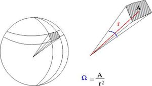
[math]\Omega[/math]= surface area of a sphere covered by the detector

ie;the detectors area projected onto the surface of a sphere

A= surface area of detector

r=distance from interaction point to detector

[math]\Omega = \frac{A}{r^2} [/math]sterradians

[math]A_{sphere} = 4 \pi r^2[/math] if your detector was a hollow ball

[math]\Omega_{max} = \frac{4 \pi r^2}{r^2} = 4\pi[/math]sterradians

Differential cross section

[math]\sigma(\theta)[/math] = [math] \frac{d \sigma}{d \Omega} \equiv \frac{\frac{\# particles\; scattered}{solid \; angle}} {\frac{ \# incident \; particles}{Area}}[/math]

Units

Cross-sections have the units of Area

1 barn = [math]10^{-28} m^2[/math]

[units of [math]\sigma(\theta)[/math]] =[math]\frac{\frac{[particles]}{[sterradian]}} {\frac{ [ particles]}{[m^2]}} = m^2[/math]

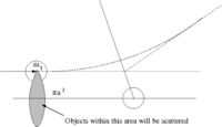
Fixed target scattering

[math]N_{in}[/math]= # of particles in = [math]I \cdot A_{in}[/math]

[math]A_{in}[/math] is the area of the ring of incident particles

[math]dN_{in} = I \cdot dA = I (2\pi b) db[/math]= # particles in a ring of radius [math]b[/math] and thickness [math]db[/math]

Scattering Length (a)

Definition

[math]a^2 = \frac{1}{4 \pi} \lim_{k \rightarrow 0} \sigma[/math]

While scattering length has the dimension of length it really represents the strength of the scattering (probability of scattering). It effectively give the amplitude of the scattered wave.

Note

the above definition is essentially an expression of how the low energy cross section corresponds to the classical value of [math]4 \pi a^2[/math]

[math]\sigma[/math] = scattering cross-section [math]\equiv \frac{\# particles\; scattered} {\frac{ \# incident \; particles}{Area}}[/math]

classically: the number of particles scattered = number of incident particles (the collision probability is unity)

Area = [math] \pi a^2[/math] = The area profile in which a collision occurs

[math]\sigma = \frac{{N}}{\frac{ N}{\pi a^2}} = \pi a^2[/math]

To derive an expression for the scattering length lets start with a general expression for a scattered wave.

A general scattered wave function has the form

[math]\Psi_g = \frac{1}{(2 \pi)^{3/2}} \left [ e^{i \vec{k} \cdot \vec{r}} + f(q) \frac{e^{ikr}}{r}\right ][/math]

The first term represents a plane wave and the second term represent a modification of the plane wave due to the scattering in terms of the scattering probability [math]|f(q)|^2[/math].

From our previous phase shift calculation, Schrodinger solutions tend to have the general form

[math]\Psi_S = \sum_{\ell} A_{\ell} P_{\ell} [\cos(\theta)] \frac{U_{\ell}(r)}{kr}[/math]

[math]= \sum_{\ell} A_{\ell} P_{\ell} [\cos(\theta)] \frac{\sin(kr - \frac{\ell \pi}{2} + \delta_{\ell})}{kr}[/math] (our previous solution was for [math]\ell=0[/math])

where

the angular part is given as

[math] P_{\ell} \cos(\theta)[/math]

and the radial part is

[math]\frac{U_{\ell}(r)}{r}[/math]

By comparing our general solution from the phase shift and our schrodinger solution we can cast f(q) in terms of the phase shift [math]\delta_{\ell}[/math] and then define the cross section as

[math]\sigma = \int |f(q)|^2 d \Omega[/math]

in order to get a gereral expression for a scattering cross section which we then take the limit of the momentum going to zero in order to get a general expression for the scattering length.

Math trick to recast plane waves

[math]e^{i\vec{k} \cdot \vec{r}} = 4 \pi \sum_{\ell m} i^{\ell} Y^*_{\ell m}(\hat{k}) Y_{\ell m}(\hat{r}) J_{\ell m}(|k| |r|)[/math]

where

[math]\hat{k}[/math] and [math]\hat{r}[/math] are the [math]\theta[/math] and [math]\phi[/math] directions of [math]\vec{k}[/math] and [math]\vec{r}[/math] respectively.

To determine the scattering length we will be looking at [math]k \rightarrow 0[/math] so let [math]\hat{k}=0 \Rightarrow \theta=0 , \phi=0[/math] use the approximation

[math]Y^*_{\ell m}(\theta=0,\phi=0) = \sqrt{\frac{2 \ell +1}{4 \pi}}\delta_{m,0}[/math]

using the above to recast [math]\Psi_g[/math] to look more like [math]\Psi_S[/math]

[math]\Psi_g = \frac{1}{(2 \pi)^{3/2}} \left \{ 4 \pi \sum_{\ell} i^{\ell} \sqrt{\frac{2 \ell +1}{4 \pi}}\delta_{m,0} Y_{\ell m}(\hat{r}) J_{\ell m}(|k| |r|) + f(q) \frac{e^{ikr}}{r} \right \}[/math]

[math]\delta_{m,0} Y_{\ell m}(\hat{r}) =Y_{\ell 0}(\hat{r}) = \sqrt{\frac{2 \ell +1}{4 \pi}} P_{\ell} [\cos(\theta)][/math]

[math]\Rightarrow \Psi_g = \frac{1}{(2 \pi)^{3/2}} \left \{ \sum_{\ell} i^{\ell} (2 \ell +1) P_{\ell} [\cos(\theta)] J_{\ell m}(|k| |r|) + f(q) \frac{e^{ikr}}{r} \right \}[/math]

which we want to compare to \Psi_S

[math]\Psi_S = \sum_{\ell} A_{\ell} P_{\ell} [\cos(\theta)] \frac{\sin(kr - \frac{\ell \pi}{2} + \delta_{\ell})}{r}[/math]

Using the identities:

[math]\sin(kr - \frac{\ell \pi}{2} + \delta_{\ell}) = \frac{e^{i(kr - \frac{\ell \pi}{2} + \delta_{\ell})} - e^{-i(kr - \frac{\ell \pi}{2} + \delta_{\ell})}}{2i}[/math]

[math]J_{\ell m}(|k| |r|) = \frac{e^{i(kr - \frac{\ell \pi}{2} )} - e^{-i(kr - \frac{\ell \pi}{2} )}}{2ir}[/math]

By equating the two solutions

[math]\Psi_S = \Psi_g[/math]

[math]e^{-ikr} \Rightarrow A_{\ell} e^{i\delta_{\ell}} = \frac{i^{\ell} (2 \ell +1)}{(2 \pi)^{3/2}}[/math]

[math]e^{+ikr} \Rightarrow [/math]

[math]\sum_{\ell} \frac{A_{\ell}}{kr} P_{\ell} [\cos(\theta)]e^{i (kr - \frac{\ell \pi}{2} + \delta_{\ell})} = \sum_{\ell} \frac{i^{\ell} (2 \ell +1)}{(2 \pi)^{3/2} 2ikr} P_{\ell} [\cos(\theta)]e^{i(kr - \frac{\ell \pi}{2} )} + \frac{f(q) e^{ikr}}{(2 \pi)^{3/2}r}[/math]

[math]\Rightarrow \frac{f(q) e^{ikr}}{(2 \pi)^{3/2}r}= \sum_{\ell} \frac{ P_{\ell} [\cos(\theta)]}{2ikr} e^{- i \ell \pi/2} \left ( \frac{A_{\ell}}{kr} e^{i (kr - \frac{\ell \pi}{2} + \delta_{\ell})} - \frac{i^{\ell} (2 \ell +1)}{(2 \pi)^{3/2}} e^{i(kr - \frac{\ell \pi}{2} )} \right ) [/math]

[math]= \sum_{\ell} \frac{A_{\ell}}{kr} e^{i (kr - \frac{\ell \pi}{2} + \delta_{\ell})} - \frac{i^{\ell} (2 \ell +1)}{(2 \pi)^{3/2} 2ikr} P_{\ell} [\cos(\theta)]e^{i(kr - \frac{\ell \pi}{2} )}[/math]

[math]\Rightarrow f(q) = \frac{1}{k} \sum_{\ell} (2 \ell + 1 ) P_{\ell} [\cos(\theta)] \sin(\delta_{\ell}) e^{i \delta_{\ell}}[/math]

[math]\sigma = \int | f(q) |^2 d \Omega[/math]

[math]= \sum_{\ell \ell^{\prime}} \int \frac{2 \ell + 1 )(2 \ell^{\prime} + 1)}{k^2}P_{\ell} [\cos(\theta)] \sin(\delta_{\ell}) e^{i \delta_{\ell}} P_{\ell^{\prime}} [\cos(\theta)] \sin(\delta_{\ell^{\prime}}) e^{-i \delta_{\ell^{\prime}}}[/math]

[math] \int P_{\ell} P_{\ell^{\prime}} d \theta = \frac{2}{2 \ell + 1} \delta_{\ell \ell^{\prime}}[/math]

[math]\Rightarrow \sigma = \frac{4 \pi}{k^2} \sum_{\ell} (2 \ell +1 ) \sin^2(\delta_{\ell})[/math]

[math]a^2 = \frac{1}{4 \pi} \lim_{k \rightarrow 0} \sigma = \frac{1}{4 \pi} \lim_{k \rightarrow 0} \frac{4 \pi}{k^2} \sum_{\ell} (2 \ell +1 ) \sin^2(\delta_{\ell})[/math]

For S-wave scattering [math]\ell =0[/math]

[math]\Rightarrow a = \pm \lim_{k \rightarrow 0} \frac{\sin(\delta_0)}{k}[/math]

To keep "a" finite the phase shift [math]\delta_{\ell}[/math] must approach zero at low energy

[math]\Rightarrow a = \pm \lim_{k \rightarrow 0} \frac{\delta_0}{k}[/math]

Singlet and Triplet States

Our previous calculation of the total cross section for nucleon nucleon scattering using a phase shift analysis gave

[math]\sigma = \frac{4 \pi}{k_2^2}\sin^2(\delta_0)[/math]

assuming [math]\ell[/math] =0.

When solving Schrodinger's equation for a neutron scattering from a proton we were left with the transcendental equation from boundary conditions

[math]\alpha \equiv k_1 cot(k_1R) = k_2 cot(k_2R + \delta)[/math]

[math]\sigma = \frac{4 \pi}{ k_2^2 + \alpha^2} \left [\cos(k_2 R) + \frac{\alpha}{k_2} \sin(k_2R)\right ][/math]

In the case of a Deuteron bound state

[math]\ell =0[/math] and [math]S=1[/math]

R = 2 fm

[math]\alpha[/math] = 0.2 /fm

when [math]k_2 \rightarrow 0[/math]

[math]\frac{\sin(k_2 R)}{k_2} = R[/math]

[math]\cos(k_2 R) = 1[/math]

then

[math]\lim_{k_2 \rightarrow 0} \sigma = \frac{4 \pi}{ 0 + (0.2)^2} \left [1 + (0.2) 2\right ] \left ( \frac{1 barn}{100 fm^2}\right)= 4.4 barns[/math]

Experimentally the cross section is quite a bit larger

[math]\sigma_{Exp}[/math] = 20.3 b

Apparently our assumption that the dominant part of the cross section is S=1 is wrong. There also exists a spin singlet (S=0) contribution to the cross section.

When the neutron and proton interact (create a bound state or an intermediate state) their spins can couple to either a net value of S=0 or S=1. There is only one component along the quantization axis in the event that they couple to an S=0 state. There are 3 possible components ([math]S_z[/math] = -1/2, 0 . + 1/2) in the event that they couple to an S=1 state.

If you sum up the two possible cross-section,[math] \sigma_S[/math] and [math]\sigma_T[/math], then you must weight them according to the possible psin compinations such that

[math]\sigma_{tot} = \frac{3}{4} \sigma_T + \frac{1}{4} \sigma_S[/math]

Solving for [math]\sigma_S \Rightarrow[/math]

[math]\sigma_S = 68[/math] barns

Because the cross sections depend on the spin date we can conclude that

The Nuclear Force is SPIN DEPENDENT

Also

Using the spatial wave functions for the singlet and triplet state one can deduce that

[math]a_T[/math] = + 6.1 fm [math]\Rightarrow[/math] there is a triplet np bound state

[math]a_S[/math] = - 23.2 fm [math]\Rightarrow[/math] there is NO singlet np bound state

Doing similar but more complicated calculations for p-p and n-n scattering results in

[math]a_{p-p}[/math] = -7.82 fm [math]\Rightarrow[/math] there is NO pp bound state

[math]a_{n-n}[/math] = -16.6 fm [math]\Rightarrow[/math] there is NO nn bound state

The Nuclear Potential

From the above we have found information on the range of the nuclear force, it's spin dependence, and it's ability to create non-spherically disrtibuted systems (quadrupole moments).

The Central Potential

No matter what potential Well geometry we choose for the nucleon, we consistently find a term which is purely radial in nature (a Central term).

[math]\lt V_c(r)\gt = \int U^*(r) V_c(r) U(r) dr = \frac{\hbar (\ell + 1) \ell}{2m} \int |U(r)|^2G(\delta) \frac{dr}{r^2} [/math]

where

[math]G(\delta)[/math] = a parameterization of[math] V_c[/math] which is constrained by scattering phase shift information.

The Spin Potential

We know from the lack of a p-p [math](^2NHe)[/math] or n-n bound system that the nuclear force is strongly spin dependent. This is reenforced even more based on our observations of the S=1 n-p bound state (the Deuteron).

Experiments also indicate that parity is conserved to the [math]10^{-7}[/math] level. [math]\Rightarrow[/math] experiments with an relative precision of [math]\frac{\Delta X}{X} \gt 10^{-7}[/math] have yet to find a parity violation.

[math]\Rightarrow[/math] The spin potential would have terms involving spin scalar quantities because a spin potential with terms that are linear combinations of spin would violate parity.

Consider a spin potential function such that the total spin is given by

[math]\vec{S} = \vec{s}_1 + \vec{2}_2[/math]

The scalar spin quantity [math]S^2[/math] would be given by

[math]\vec{S} \cdot \vec{S} = s_1^2 + 2\vec{s}_1 \cdot \vec{s}_2 + s_2^2[/math]

or

[math]\vec{s}_1 \cdot \vec{s}_2 = S^2 -s_1^2-s_2^2[/math]

Spin Singlet

if

S=0

then

[math]\lt \vec{s}_1 \cdot \vec{s}_2 \gt = \lt S^2\gt -\lt s_1^2\gt -\lt s_2^2\gt [/math]

[math]= \left [ S(S+1) - s_1(s_1+1) - s_2(s_2+1) \right ] \frac{\hbar^2}{2}[/math]

[math]= \left [ 0(0+1) - \frac{1}{2} (\frac{1}{2}+1)- \frac{1}{2} (\frac{1}{2}+1)\right ] \frac{\hbar^2}{2}[/math]

[math]= - \frac{3}{4} \hbar^2[/math]

Spin Triplet

if

S=1

then

[math]\lt \vec{s}_1 \cdot \vec{s}_2 \gt = \lt S^2\gt -\lt s_1^2\gt -\lt s_2^2\gt [/math]

[math]= \left [ S(S+1) - s_1(s_1+1) - s_2(s_2+1) \right ] \frac{\hbar^2}{2}[/math]

[math]= \left [ 1(1+1) - \frac{1}{2} (\frac{1}{2}+1)- \frac{1}{2} (\frac{1}{2}+1)\right ] \frac{\hbar^2}{2}[/math]

[math]= + \frac{1}{4} \hbar^2[/math]

Construct the Spin Potential

Let

V_1(r) = spin singlet parameterized potential

V_3(r) = spin triplet parameterized potential

Then

V_s(r) = - (

Nuclear Models

Given the basic elements of the nuclear potential from the last chapter, one may be tempted to construct the hamiltonian for a group of interacting nucleons in the form

[math]H = \sum_i^A T_i + \sum_i\lt j^A V_{ij}[/math]

where

[math]T_i[/math] represent the kinetic energy of the ith nucleon

[math]V_{ij}[/math] represents the potential energy between two nucleons.

If you assume that the nuclear force is a two body force such that the force between any two nucleons doesn't change with the addition of more nucleons, Then you can solve the Schrodinger equation corresponding to the above Hamiltonian for A<5.

For A< 8 there is a technique called Green's function monte carlo which reportedly finds solution that are nearly exact. J. Carlson, Phys. Rev. C 36, 2026 - 2033 (1987), B. Pudliner, et. al., Phys. Rev. Lett. 74, 4396 - 4399 (1995)

Shell Model

Independent particle model

This part of the Shell model suggests that the properties of a nucleus with only one unpaired nucleon are determined by that one unpaired nucleon. The unpaired nucleon usually, though no necessarily, occupies the outer most shell as a valence nucleon.

SN-130 Example

The low lying excited energy states for Sn-130 taken from the LBL website are given below.

File:Sn-130 LowLyingE Levels.tiff

The listing indicates that the ground state of Sn-130 is a spin 0 positive parity [math](J^{\pi} = 0^+)[/math] state. The first excited state of this nucleus is 1.22 MeV above the ground state and has [math](J^{\pi} = 2^+)[/math]. The next excited state is 1.95 MeV above the ground state and has [math](J^{\pi} = 7^-)[/math].

Let's see how well the shell model does at predicting these [math](J^{\pi} )[/math] states

Liquid Drop Model

Bohr and Mottelson considered the nucleon in terms of its collective motion with vibrations and rotations that resembled a suspended drop of liquid.

Nuclear Reactions

Types of Reactions

[math]a + X \rightarrow Y + b[/math]

elastic scattering

X & Y and a & b are the same particles, momentum and energy are conserved, typically all are in their ground state

In-elastic scattering

Nuclear Decay

Alpha Decay

The spontaneous emission of an alpha particle[math]({4\atop 2 }He_{2})[/math] is the result of a natural decay process which can be described as the tunneling of energy ( in the form of the alpha particle) through the coulomb barrier. In other words, if a collection of nucleons within a nucleus finds itself sufficiently close to the nuclear force potential well limit, then a coulomb repulsion force can begin to dominant and facilitate the tunneling of this collection of nucleons ( an alpha particle) through the confining potential well.

The decay process can be represented by the following reaction notation

[math]{A \atop Z }X_{N} \rightarrow {A-4 \atop Z-2 }Y_{N-2} + \alpha[/math]

Q-value

The "Q-value" represents the net mass energy released in a nuclear reaction.

In the above example the Q value is calculated :

[math]E_i = E_f[/math]

[math]m_Xc^2 +T_X = m_Yc^2 + T_Y + m_{\alpha}c^2 + T_{\alpha}[/math]

[math]T_X = 0[/math] : assume nucleus is initially at rest

[math]Q \equiv m_Xc^2 -m_Yc^2 - m_{\alpha}c^2 = T_Y + T_{\alpha}[/math]

Example

[math]{232 \atop 92 }U_{140} \rightarrow {228 \atop 90 }Th_{138} + \alpha[/math]

[math]Q = (232.0371463 - 228.0287313 - 4.002603 )uc^2 \frac{931.502 MeV}{uc^2} = 5.414 MeV[/math]

The positive Q value (Q>0) identifies the reaction as exothermic (exoergonic) which means that energy is given off and that the reaction is spontaneous

A negative Q value (Q<0) identifies the reaction as endothermic (endoergonic) which means that energy is required to for the reaction to take place.

Kinetic energy of alpha

Since the original nucleus was at rest, the final nuclei will have the same momentum in opposite directions in order to conserve momentum.

[math]T_{Y} = \frac{p^2_{Y}}{2m_Y}= \frac{p^2_{\alpha}}{2m_Y} = T_{\alpha} \frac{m_{\alpha}}{m_Y}[/math]

[math]Q = = T_Y + T_{\alpha} = T_{\alpha} \left ( \frac{m_{\alpha}}{m_Y} + 1\right )[/math]

[math]=T_{\alpha} \left ( \frac{4}{A-4} + 1\right ) = T_{\alpha} \left ( \frac{A}{A-4} \right )[/math]

[math] \Rightarrow T_{\alpha} = Q \left (1- \frac{4}{A} \right )[/math]

Example

[math]{232 \atop 92 }U_{140} \rightarrow {228 \atop 90 }Th_{138} + \alpha[/math]

[math] T_{\alpha} = Q \left (1- \frac{4}{A} \right )= 5.414 MeV \left (1- \frac{4}{228} \right ) = 5.32 MeV[/math]

The alpha particle caries away most of the kinetic energy.

Kinetic energy of alpha

Geiger-Nuttal Law

In 1911 Geiger and Nuttal noticed that the decay half life ([math]T_{1/2})[/math] of nuclei that emmitt alpha particles was related to the disentegration energy [math](Q)[/math].

[math]\log_{10}(T_{1/2}) = a + \frac{b}{\sqrt{Q}}[/math]

It works best for Nuclei with Even [math]Z[/math] and Even[math] N[/math]. The trend is still there for Even-Odd, Odd-Even, and Odd-odd nuclei but not as pronounced.

cluster decays

The Gieger-Nuttal Law has been extended to describe the decay of Large A (even-even and odd A) nuclei into clusters in which Silicon or Carbon are one of the clusters.

http://prola.aps.org/pdf/PRC/v70/i3/e034304

Homework problems

NucPhys_I_HomeworkProblems

Midterm Exam Topics list

Basically everything before section 5.3 (The Nuclear Force). Section 5.3 and below is not included on the midterm.

Topics of emphasis:

1. 1-D Schrodinger Equation based problems involving discrete potentials ( wells, steps) and continuous potentials (simple Harmonic, coulomb).
2. Calculating form factors given the density of a nucleus
3. Determining binding and nucleon mass separation energies
4. [math]\vec{I}[/math], [math]\vec{\ell}[/math], and [math]\vec{s}[/math] angular momentum operations
5. Calculating scattering rates given the cross-section and a description of the experimental apparatus

Formulas given on test

Schrodinger Time independent 1-D equation

[math]\left ( \frac{- \hbar^2}{2m} \frac{ \part^2}{\part x^2} + V \right ) \psi = E \psi[/math]

Particle Current Density

[math]j = \frac{ \hbar}{2im} \left ( \Psi^* \frac{\part \Psi}{\part x} - \Psi \frac{\part \Psi^*}{\part x}\right )[/math]

Form Factor

If the density has no [math]\theta[/math] or [math]\phi[/math] dependence

[math]F(q) = \frac{4 \pi}{q} \int \sin(qr) \rho(r) rdr[/math]

Coulomb energy difference between point nucleus and one with uniform charge distribution

[math]\Delta E = \frac{2}{5} \frac{Z^4e^2}{4 \pi \epsilon_0} \frac{R^2}{a_0^3}[/math]

Nucleus Binding Energy

[math]B(^A_ZX_N) = \left [ Z m(^1H) + Nm_n -m(^AX) \right ]c^2[/math]

Neutron Separation energy

[math]S_n = B(^A_ZX_N) - B(^{A-1}_ZX_{N-1})[/math]

Proton Separation energy

[math]S_p = B(^A_ZX_N) - B(^{A-1}_{Z-1}X_N)[/math]

Semiempirical Mass Formula

[math]M(Z,A) = Z m(^1H) + Nm_n - B(^A_ZX_N)/c^2[/math]

where

[math]B(^A_ZX_N) = = \alpha_V A - \alpha_S A^{2/3} - \alpha_C \frac{Z(Z-1)}{A^{1/3}} - \alpha_{sym} \frac{(A-2Z)^2}{A} - \delta[/math]

Parameter	Krane
[math]\alpha_V[/math]	15.5
[math]\alpha_S[/math]	16.8
[math]\alpha_C[/math]	0.72
[math]\alpha_{sym}[/math]	23
[math]\alpha_p[/math]	[math]\pm[/math]34

[math]g_{\ell} =\left \{ {1 \;\;\;\; proton \atop 0 \;\;\;\; neutron} \right .[/math]

[math]g_{s} =\left \{ {5.5856912 \pm 0.0000022 \;\;\;\; proton \atop -3.8260837 \pm 0.0000018 \;\;\;\; neutron} \right .[/math]

Final

1.) Calculate the magnetic moment of a proton assuming that it may be described as a neutron with a positive pion [math](\pi^+)[/math] in an [math]\ell =1[/math] state.

2.) Show that the phase shift ([math]\delta_0[/math]) for the scattering of a neutron by a proton can be given by the equation

[math]\delta_0 = \tan^{-1} \left( \frac{\tan(k_1R) - \frac{k_1}{k_2} \tan(k_2R)}{ \tan(k_1R) \tan(k_2R)+\frac{k_1}{k_2}}\right )[/math]

where

[math]k_1^2 = \frac{2m(V+E)}{\hbar^2}[/math]

[math]k_2^2 = \frac{2mE)}{\hbar^2}[/math]

V = 36.7 MeV R = 2.1 fm

3.)

a.) Write the reaction equations for the following processes. Show all reaction products.

i.)[math]{226 \atop\; }Ra \; \; \; \alpha - decays[/math]

ii.)[math]{110 \atop\; }In \; \; \; \beta^+ - decays[/math]

iii.)[math]{36 \atop\; }Ar (2^{nd} 0^{+}) \; \; \; internal conversion[/math]

iv.)[math]{12 \atop\; }C (2^+) \; \; \; \gamma - decays[/math]

b.) Determine the Q-values for the first two reactions above.

4.) Find the Quadrupole moment of [math]{209 \atop\; }Bi(9/2^-)[/math] using the shell model and compare to the experimental value of -0.37 barns.

5.) Find [math]\frac{\mu}{\mu_{NM}}[/math], using the shell model, for the following nuclei

a.)[math] {75 \atop\; }Ge[/math]

b.) [math]{87 \atop\; }Sr[/math]

c.) [math]{91 \atop\; }Zr[/math]

d.) [math]{47 \atop\; }Sc[/math]

6.) Use the shell model to predict the ground state spin and parity of the following nuclei:

a.) [math]{7 \atop\; }Li[/math]

b.)[math] {11 \atop\; }B[/math]

c.) [math]{15 \atop\; }C[/math]

d.)[math] {17 \atop\; }F[/math]

7.) Tabulate the possible [math]m[/math] states for a nucleus three quadrupole phonon state ([math]\lambda = 3[/math] ). Show that the permitted resultant states are [math]0^+[/math], [math]2^+[/math], [math]3^+[/math], [math]4^+[/math], and [math]6^+[/math].