|
|
| Line 188: |
Line 188: |
| | ::<math>= \frac{16e^4}{(p_1-p_2)^4} \left [ (p_2\cdot p_3) (p_1 \cdot p_4) + (p_2 \cdot p_4 ) (p_1 \cdot p_3) + 0 \right ]</math> | | ::<math>= \frac{16e^4}{(p_1-p_2)^4} \left [ (p_2\cdot p_3) (p_1 \cdot p_4) + (p_2 \cdot p_4 ) (p_1 \cdot p_3) + 0 \right ]</math> |
| | :::<math>+ \left [ (p_1\cdot p_3) (p_2 \cdot p_4) + (p_1\cdot p_4) (p_2\cdot p_3) + 0 \right ]</math> | | :::<math>+ \left [ (p_1\cdot p_3) (p_2 \cdot p_4) + (p_1\cdot p_4) (p_2\cdot p_3) + 0 \right ]</math> |
| − | :::<math>+ 4\left ( m_2m_1m_3m_4 - (p_2 \cdot p_1 )m_3m_4 - m_2m_1(p_3 \cdot p_4\right ) \right ]</math> | + | :::<math>+ 4\left [ m_2m_1m_3m_4 - (p_2 \cdot p_1 )m_3m_4 - m_2m_1(p_3 \cdot p_4) \right ]</math> |
| | | | |
| | =e+e- Annihilation (s-channel) (time-like)= | | =e+e- Annihilation (s-channel) (time-like)= |
Revision as of 04:55, 17 April 2012
Bhabha (electron - positron) Scattering
Bhabha scattering identifies the scatterng of an electron and positron (particle and anti-particle). There are two processes that can occur
1.) scattering via the "instantaneous" exchange of a virtual photon
2.) annihilation in which the e+ and e- spend some time as a photon which then reconverts back to an e+e- pair
e+e- scattering (t-channel) (space-like)
The Feynman diagram is a space-time description of the interaction where the horizontal axis (abscissa) is used to denote time and the vertical axis (ordinate) is 3-D space.
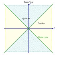
A particle which travels only along the horizontal time axis is not moving in space while a particle traveling only along the vertical axis is not moving in time (within the uncertainty principle).
Step 1 Draw the Feynman Diagram
If the electron and positron simply scatter off of one another via a coulomb interaction, then they exchange a photon along the space axis. You start with an external line from the left to represent the electron. This is a "t-channel" process in which one of the particles emits a virtual photon that is absorbed by the other particle (the internal photon connects two vertices). You can tell the exchanged particle is virtual if it is drawn parallel to the time axis in the Feynman diagram.
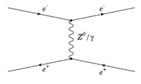
- The time axis is from left to right so the Virtual particle is along the space axis (in some books the diagram has the space axis horizontal). Also note that a virtual, neutral Z-boson may also be exchanged via the electro-weak interaction.
Step 2 Label 4-Momentum
Let:
- [math]p_1=p_{in}(e^-) \equiv[/math] initial electron 4-momentum
- [math]u_1 \equiv[/math] initial electron spinor
- [math]p_2=p_{out}(e^-) \equiv[/math] final electron 4-momentum
- [math]u_2 \equiv[/math] final electron spinor
- [math]p_3= p_{in}(e^+) \equiv[/math] initial positron 4-momentum
- [math]\bar{u}_3 \equiv[/math] initial positron spinor
- [math]p_4 = p_{out}(e^+) \equiv[/math] final positron 4-momentum
- [math]\bar{u}_4 \equiv[/math] final positron spinor
Momentum conservation at the electron vertex
Conservation of 4-momentum at the electron vertex for the e+e- scattering Feynman diagram
- [math]p^{\mu}_{in}(e^-) = p^{\mu}_{out}(\gamma^*) + p^{\mu}_{out}(e^-) [/math]
- [math]\Rightarrow p^{\mu}_{out}(\gamma^*) = p^{\mu}_{in}(e^-) - p^{\mu}_{out}(e^-) [/math]
- [math] q^{\mu} = (E_{\gamma},\vec{p_{\gamma}})= (E_1,\vec{p}_1) - (E_2,\vec{p}_2) = (E_1-E_2,\vec{p}_1 - \vec{p}_2)[/math]
- [math]q^2 = q_{\mu}q^{\mu}= (E_1-E_2,-(\vec{p}_1 - \vec{p}_2)) (E_1-E_2,\vec{p}_1 - \vec{p}_2)= (E_1-E_2)^2-(\vec{p}_1 - \vec{p}_2) \cdot (\vec{p}_1 - \vec{p}_2)[/math]
- [math] = (E_1-E_2)^2-p_1^2 -p_2^2 + 2p_1p_2 \cos(\theta)[/math]
- [math] = E_1^2 - p_1^2 +E_2^2 - p_2^2 - 2E_1E_2+ 2p_1p_2 \cos(\theta)[/math]
- [math] = m_1^2 + m_2^2- 2(E_1E_2- p_1p_2 \cos(\theta))[/math]
- [math]m_{\gamma}^2=E_{\gamma}^2 - p_{\gamma}^2= m_1^2 + m_2^2 -4p_1p_2\sin^2(\theta/2)[/math]
if
- [math]E_{\gamma}^2 - p_{\gamma}^2= m_1^2 + m_2^2 -4p_1p_2\sin^2(\theta/2) \ne 0[/math]
Then
- [math]m_{\gamma}^2 \ne 0 \Rightarrow[/math] photon with mass [math]\Rightarrow[/math] Virtural Photon
Step 3 Matrix Element
electron emits photon Vertex
The electron scatters
- [math]\bar{u}_2 (ig_e\gamma^{\mu} )u_1[/math]
photon propogator
- [math]\left ( \frac{-ig_{\mu \nu}}{(p_1-p_2)^2} \right)[/math]
where
- [math]q^2 = E_1^2 - p_1^2 +E_2^2 - p_2^2 - 2E_1E_2+ 2p_1p_2 \cos(\theta)[/math]
- [math] = m_1^2 + m_2^2- 2(E_1E_2- p_1p_2 \cos(\theta))[/math]
- [math]= m_1^2 + m_2^2 -4p_1p_2\sin^2(\theta/2)[/math]
Positron absorbs photn Vertex
The positron absorbs the photon emitted by the electron
- [math]\bar{u}_3 (ig_e\gamma^{\nu} ) u_4[/math]
- because of the arrow for anti-particles the final state u_4 appears on the most left hand side as the initial state.
Matrix amplitude
The Matrix element is a product of the vertex and propagator terms
- [math]\mathcal{M}_t = \bar{u}_2 (ig_e\gamma^{\mu}) u_1 \left ( \frac{-ig_{\mu \nu}}{(p_1-p_2)^2} \right) \bar{u}_3 (ig_e \gamma^{\nu}) u_4[/math] = t-channel scattering matrix amplitude
- [math] = \bar{u}_2 (ig_e\gamma^{\mu}) u_1 \left ( \frac{1}{(p_1-p_2)^2} \right) \bar{u}_3 (ig_e \gamma_{\mu}) u_4[/math]
- [math] = \left ( \frac{-g_e^2}{(p_1-p_2)^2} \right) [\bar{u}_2 \gamma^{\mu} u_1] [\bar{u}_3 \gamma_{\mu} u_4][/math]
[math]|\mathcal{M}_t |^2 = \frac{e^4}{(p_1-p_2)^4} \Big( [\bar{u}_2 \gamma^{\mu} u_1] [\bar{u}_3 \gamma_{\mu} u_4]\Big)^* \Big( ([\bar{u}_2 \gamma^{\mu} u_1] [\bar{u}_3 \gamma_{\mu} u_4]\Big) [/math]
- [math]= \frac{e^4}{(p_1-p_2)^4} \Big( (\bar{u}_1 \gamma^\mu u_2 ) ( \bar{u}_4 \gamma_\mu u_3) \Big) \Big( (\bar{u}_2 \gamma^\nu u_1)( \bar{u}_3 \gamma_\nu u_4 \Big )[/math](complex conjugate will flip order)
- [math]= \frac{e^4}{(p_1-p_2)^4} \Big( (\bar{u}_1 \gamma^\mu u_2 ) (\bar{u}_2 \gamma^\nu u_1)( \bar{u}_4 \gamma_\mu u_3)( \bar{u}_3 \gamma_\nu u_4 \Big)[/math] (move terms that depend on same momentum to be next to each other)
Spin averaged matrix element
To determine actual cross-sections and lifetimes you need to insert the specific spinors for the physics process
- or you can overage over all the initial spin states and sum over all the final spin states to determine the cross section.
[math]\lt \left | \mathcal{M}^2 \right | \gt \equiv[/math] average over all intial spin states and sum over all the final spin states for [math]\left | \mathcal{M} \right |^2[/math]
- [math]= \frac{e^4}{(p_1-p_2)^4} \sum_{s_1} \left ( \bar{u}_1 \gamma^\mu \left [ \sum_{s_2} u_2 \bar{u}_2 \right ]\gamma^\nu u_1 \right) \sum_{s_4} \left ( \bar{u}_4 \gamma_\mu \left [ \sum_{s_3} u_3\bar{u}_3 \right ] \gamma_\nu u_4 \right )[/math]
Working with the first set of matrices
- [math]\sum_{s_1} \left ( \bar{u}_1 \gamma^\mu \left [ \sum_{s_2} u_2 \bar{u}_2 \right ]\gamma^\nu u_1 \right)[/math]
- The completeness relation
- [math]\sum_{s_2} u_2 \bar{u}_2 = p\!\!\!/_2 + m_2 [/math]
Let
- [math]Q = \gamma^\mu \left ( p\!\!\!/_2 + m_2 \right ) \gamma^\nu[/math] a 4 x 4 matrix
Then
- [math]\sum_{s_1} \left ( \bar{u}_1 \gamma^\mu \left [ \sum_{s_2} u_2 \bar{u}_2 \right ]\gamma^\nu u_1 \right) =\sum_{s_1} \left ( \bar{u}_1 Q u_1 \right)[/math]
- [math]= \sum_{s_1} (\bar{u}_1)_i Q_{ij} (u_1)_j [/math]
- [math]= Q_{ij} \left ( \sum_{s_1} u_1 \bar{u}_1 \right )_{ji} [/math] property of matrices
- [math]= Q_{ij} \left ( ( p\!\!\!/_1 + m_1) \right )_{ji} [/math] completeness relation
- [math]= \left ( Q ( p\!\!\!/_1 + m_1) \right )_{ii}[/math]
- [math]= Tr\left [ Q ( p\!\!\!/_1 + m_1) \right][/math]: Def of trace is the sum of diagonal elements in a matrix
- [math]= Tr\left [ \gamma^\mu \left ( p\!\!\!/_2 + m_2 \right ) \gamma^\nu ( p\!\!\!/_1 + m_1) \right][/math]:
Evaluating the Matrix element in terms of Traces
Using the above relation for the matrix element
- [math]\mathcal{M_t}= \frac{e^4}{(p_1-p_2)^4} \sum_{s_1} \left ( \bar{u}_1 \gamma^\mu \left [ \sum_{s_2} u_2 \bar{u}_2 \right ]\gamma^\nu u_1 \right) \sum_{s_4} \left ( \bar{u}_4 \gamma_\mu \left [ \sum_{s_3} u_3\bar{u}_3 \right ] \gamma_\nu u_4 \right )[/math]
- [math]= \frac{e^4}{(p_1-p_2)^4} Tr\left [ \gamma^\mu \left ( p\!\!\!/_2 + m_2 \right ) \gamma^\nu ( p\!\!\!/_1 + m_1) \right] Tr\left [ \gamma_\mu \left ( p\!\!\!/_3 + m_3 \right ) \gamma_\nu ( p\!\!\!/_4 + m_4) \right][/math]
- [math]Tr\left [ \gamma^\mu \left ( p\!\!\!/_2 + m_2 \right ) \gamma^\nu ( p\!\!\!/_1 + m_1) \right] =[/math]
- [math]Tr\left [ \gamma^\mu p\!\!\!/_2 \gamma^\nu p\!\!\!/_1 \right] +Tr\left [ \gamma^\mu p\!\!\!/_2 \gamma^\nu m_1 \right] +Tr\left [ \gamma^\mu m_2 \gamma^\nu p\!\!\!/_1\right] + Tr\left [ \gamma^\mu m_2 \gamma^\nu m_1\right][/math]
- [math]Tr\left [ \gamma^\mu p\!\!\!/_2 \gamma^\nu m_1 \right] +Tr\left [ \gamma^\mu m_2 \gamma^\nu p\!\!\!/_1\right] = 0[/math] : The trace of a product with an odd number of [math] \gamma[/math] matrices is zero (remember [math]p\!\!\!/ = \gamma^{\mu} p_{\mu}[/math]).
- [math]Tr\left [ \gamma^\mu \left ( p\!\!\!/_2 + m_2 \right ) \gamma^\nu ( p\!\!\!/_1 + m_1) \right] =Tr\left [ \gamma^\mu p\!\!\!/_2 \gamma^\nu p\!\!\!/_1 \right] + Tr\left [ \gamma^\mu m_2 \gamma^\nu m_1\right][/math]
- [math]=Tr\left [ \gamma^{\mu}\gamma^{\lambda} (p_2)_{\lambda} \gamma^{\nu} \gamma^{\rho} (p_1)_{\rho} \right] + m_2m_1Tr\left [ \gamma^\mu \gamma^\nu \right][/math]
- [math]= (p_2)_{\lambda} (p_1)_{\rho} Tr\left [ \gamma^{\mu}\gamma^{\lambda} \gamma^{\nu} \gamma^{\rho} \right] + m_2m_1Tr\left [ \gamma^\mu \gamma^\nu \right][/math]
Applicable Trace identities
- [math]Tr\left [ \gamma^\mu \gamma^\nu \right] = 4g^{\mu \nu} = 4
\begin{bmatrix}
1 & 0 & 0 & 0\\
0 & -1 & 0 & 0\\
0 & 0 & -1 & 0\\
0 & 0 & 0 & -1
\end{bmatrix}
[/math]
- [math]Tr\left [ \gamma^{\mu}\gamma^{\lambda} \gamma^{\nu} \gamma^{\rho} \right] = 4 (g^{\mu \lambda} g^{\nu \rho} - g^{\mu \nu} g^{\lambda \rho} + g^{\mu \rho} g^{\lambda \nu} )[/math]
- [math](p_2)_{\lambda} (p_1)_{\rho} Tr\left [ \gamma^{\mu}\gamma^{\lambda} \gamma^{\nu} \gamma^{\rho} \right] = (p_2)_{\lambda} (p_1)_{\rho} 4 (g^{\mu \lambda} g^{\nu \rho} + g^{\mu \nu} g^{\lambda \rho} + g^{\mu \rho} g^{\lambda \nu} )[/math]
- [math] = 4\left [ (p_2)_{\lambda} (p_1)_{\rho} g^{\mu \lambda} g^{\nu \rho} - (p_2)_{\lambda} (p_1)_{\rho} g^{\mu \nu} g^{\lambda \rho} + (p_2)_{\lambda} (p_1)_{\rho}g^{\mu \rho} g^{\lambda \nu} \right ][/math]
- [math] = 4\left [ (p_2)^{\mu} (p_1)^{\nu} - g^{\mu \nu} \left ( p_2 \cdot p_1) \right ) + (p_1)^{\mu} (p_2)^{\nu} \right ][/math]
- [math]Tr\left [ \gamma^\mu \left ( p\!\!\!/_2 + m_2 \right ) \gamma^\nu ( p\!\!\!/_1 + m_1) \right] =Tr\left [ \gamma^\mu p\!\!\!/_2 \gamma^\nu p\!\!\!/_1 \right] + Tr\left [ \gamma^\mu m_2 \gamma^\nu m_1\right][/math]
- [math]= (p_2)_{\lambda} (p_1)_{\rho} Tr\left [ \gamma^{\mu}\gamma^{\lambda} \gamma^{\nu} \gamma^{\rho} \right] + m_2m_1Tr\left [ \gamma^\mu \gamma^\nu \right][/math]
- [math]= 4\left [ (p_2)^{\mu} (p_1)^{\nu} - g^{\mu \nu} \left ( p_2 \cdot p_1) \right ) + (p_1)^{\mu} (p_2)^{\nu} \right ]+ m_2m_14g^{\mu \nu}[/math]
- [math]= 4\left [ (p_2)^{\mu} (p_1)^{\nu} + (p_1)^{\mu} (p_2)^{\nu} + g^{\mu \nu} \left ( m_2m_1- p_2 \cdot p_1 \right )\right ][/math]
Insering all terms
- [math]\mathcal{M_t} =\frac{e^4}{(p_1-p_2)^4} Tr\left [ \gamma^\mu \left ( p\!\!\!/_2 + m_2 \right ) \gamma^\nu ( p\!\!\!/_1 + m_1) \right] Tr\left [ \gamma_\mu \left ( p\!\!\!/_3 + m_3 \right ) \gamma_\nu ( p\!\!\!/_4 + m_4) \right][/math]
- [math]=\frac{e^4}{(p_1-p_2)^4} 4\left [ (p_2)^{\mu} (p_1)^{\nu} + (p_1)^{\mu} (p_2)^{\nu} + g^{\mu \nu} \left ( m_2m_1- p_2 \cdot p_1 \right )\right ] [/math]
- [math]\times 4\left [ (p_3)_{\mu} (p_4)_{\nu} + (p_4)_{\mu} (p_3)_{\nu} + g_{\mu \nu} \left ( m_3m_4- p_3 \cdot p_4 \right )\right ][/math]
- [math]= \frac{16e^4}{(p_1-p_2)^4} (p_2)^{\mu} (p_1)^{\nu} \left [ (p_3)_{\mu} (p_4)_{\nu} + (p_4)_{\mu} (p_3)_{\nu} + g_{\mu \nu} \left ( m_3m_4- p_3 \cdot p_4 \right ) \right ][/math]
- [math]+(p_1)^{\mu} (p_2)^{\nu} \left [ (p_3)_{\mu} (p_4)_{\nu} + (p_4)_{\mu} (p_3)_{\nu} + g_{\mu \nu} \left ( m_3m_4- p_3 \cdot p_4 \right ) \right ][/math]
- [math]+ g^{\mu \nu} \left ( m_2m_1- p_2 \cdot p_1 \right ) \left [ (p_3)_{\mu} (p_4)_{\nu} + (p_4)_{\mu} (p_3)_{\nu} + g_{\mu \nu} \left ( m_3m_4- p_3 \cdot p_4 \right ) \right ][/math]
- [math]= \frac{16e^4}{(p_1-p_2)^4} \left [ (p_2\cdot p_3) (p_1 \cdot p_4) + (p_2 \cdot p_4 ) (p_1 \cdot p_3) + 0 \right ][/math]
- [math]+ \left [ (p_1\cdot p_3) (p_2 \cdot p_4) + (p_1\cdot p_4) (p_2\cdot p_3) + 0 \right ][/math]
- [math]+ 4\left [ m_2m_1m_3m_4 - (p_2 \cdot p_1 )m_3m_4 - m_2m_1(p_3 \cdot p_4) \right ][/math]
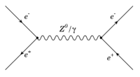
e+e- Annihilation (s-channel) (time-like)
Step 1 Draw the Feynman diagram
If the electron and positron form an intermediate state which then decays back to an electron and positron. This is an "s-channel" process in which an intermediate state is created.
Step 2 identify 4-Momentum conservation
- Momentum conservation at the first vertex
- [math]p^{\mu}_{1}(e^-) + p^{\mu}_{3}(e^+) = p^{\mu}_{out}(\gamma) [/math] Unlike scattering the e- state combines with the e+ state to emit a photon which will then produce an e+e- pair some time later. So the initial 4-momentum of the two incident particles combines to form the 4-momentum of the intermediate state
Let:
- [math]p_1 \equiv[/math] initial electron 4-momentum
- [math]u_1 \equiv[/math] initial electron spinor
- [math]p_2 \equiv[/math] final electron 4-momentum
- [math]u_2 \equiv[/math] final electron spinor
- [math]p_3 \equiv[/math] initial positron 4-momentum
- [math]\bar{u}_3 \equiv[/math] initial positron spinor
- [math]p_4 \equiv[/math] finial positron 4-momentum
- [math]\bar{u}_4 \equiv[/math] finial positron spinor
Step 3 Matrix Element
First electron positron annihilation Vertex
Initially an electron annihilates with a positron to form a photon
- [math]\bar{u}_4 (ig_e\gamma^{\mu} )u_1[/math]
photon propogator
- [math]\left ( \frac{-ig_{\mu \nu}}{(p_1+p_3)^2} \right)[/math]
reconversion Vertex
The photon converts back into an electron-positron pair
- [math]\bar{u}_3 (ig_e\gamma^{\nu} ) u_2[/math]
Matrix amplitude and magnitude
- [math]M_t = \bar{u}_3 (ig_e\gamma^{\mu}) u_2 \left ( \frac{-ig_{\mu \nu}}{(p_1+p_3)^2} \right) \bar{u}_4 (ig_e \gamma^{\nu}) u_1[/math] = s-channel annihilation matrix amplitude
- [math] = \bar{u}_3 (ig_e\gamma^{\mu}) u_2 \left ( \frac{1}{(p_1+p_3)^2} \right) \bar{u}_4 (ig_e \gamma_{\mu}) u_1[/math]
- [math] = \left ( \frac{g_e^2}{(p_1+p_3)^2} \right) [\bar{u}_3 (\gamma^{\mu}) u_2] [\bar{u}_4 ( \gamma_{\mu}) u_1][/math]
Step 4 Find total amplitude
- [math]\mathcal{M}_t = \bar{u}_2 (ig_e\gamma^{\mu}) u_1 \left ( \frac{-ig_{\mu \nu}}{(p_1-p_2)^2} \right) \bar{u}_3 (ig_e \gamma^{\nu}) u_4[/math] = t-channel scattering matrix amplitude
- [math]\mathcal{M}_s = \bar{u}_4 (ig_e\gamma^{\mu}) u_2 \left ( \frac{-ig_{\mu \nu}}{(p_1-p_2)^2} \right) \bar{u}_3 (ig_e \gamma^{\nu}) u_1[/math] = s-channel annihilation matrix amplitude
The overall amplitude ([math]\mathcal{M}_{tot}[/math]) is the coherent sum of the individual amplitudes. In the case of annihaltion (s-channel) the Feynman diagram depicts particle becoming anti-particles and the reverser. A "-" sign is introduced to "Asymmetrize" the amplitude and account for particles simply interchanging with their anti-particle.
[math]\mathcal{M}_{tot} = \mathcal{M}_t - \mathcal{M}_s[/math]
Matrix element for scattering
According to the Feynman RUles for QED:
the term
[math]ig_e \gamma^{\mu}[/math]
is used at the vertex to describe the Quantum electrodynamic (electromagneticc) interaction between the two fermion spinor states entering the vertex and forming a photon which will "connect" this vertex with the next one.
- The QED interaction Lagrangian is
- [math]-eA_{\mu} \bar{\Psi} \gamma^{\mu} \Psi[/math]
[math]\mathcal{M}_s = \,[/math]
[math]e^2 \left( \bar{u}_{3} \gamma^\nu u_4 \right) \frac{1}{(p_1+p_2)^2} \left( \bar{u}_{2} \gamma_\nu u_{1} \right) [/math]
Matrix element for annihilation
[math]\mathcal{M}_a = \,[/math]
[math]-e^2 \left( \bar{u}_{3} \gamma^\mu u_{1} \right) \frac{1}{(p_1-p_3)^2} \left( \bar{u}_{2} \gamma_\mu u_4 \right) [/math]
Radiative Bhabha Scattering to measure running of alpha
http://arxiv.org/pdf/hep-ex/0105065.pdf
Forest_QMII


