Difference between revisions of "EG1 Teleconferences DeltaDoverD"
(New page: =15-1-09=) |
|||
| Line 1: | Line 1: | ||
=15-1-09= | =15-1-09= | ||
| + | ==Cherenkov== | ||
| + | ===Cherenkov Theory=== | ||
| + | |||
| + | When the velocity of a charged particle is greater than the local phase velocity of light or when it enters a medium with different optical properties the charged particle will emit photons. The Cherenkov light is emitted under a constant angle <math>\theta_c</math> - the angle of Cherenkov radiation relative to the particle's direction. It can be shown geometrically that the cosine of the Cherenkov radiation angle is anti-proportional to the velocity of the charged particle<br> | ||
| + | |||
| + | <math>cos \theta_c=\frac{1}{n \beta}</math><br> | ||
| + | |||
| + | where <math>\beta c</math> is the particle's velocity and n - index of refraction of the medium.The charged particle in time t travels <math>\beta c t</math> distance, while the electromagnetic waves - <math>\frac{c}{n}t</math>. For a medium with given index of refraction n there is a threshold velocity <math>\beta_{thr}=\frac{1}{n}</math>, below <math>\beta_{thr}</math> no radiation can take place. This process may be used to observe the passage of charged particles in a detector which can measure the produced photons.<br> | ||
| + | |||
| + | The number of photons produced per unit path length of a particle with charge ze and per unit energy interval of the photons is proportional to the sine of the Cherenkov angle[http://pdg.lbl.gov/2007/reviews/passagerpp.pdf] <br> | ||
| + | |||
| + | <math>\frac{d^2 N}{dEdx}=\frac{\alpha z^2}{\hbar c}sin ^2 \theta_c=\frac{\alpha z^2}{\hbar c}[1-\frac{1}{\beta^2 n^2 (E)}]</math><br> | ||
| + | |||
| + | |||
| + | <math>\frac{d^2 N}{d\lambda dx} = \frac{2 \pi \alpha z^2}{\lambda^2}[1-\frac{1}{\beta^2 n^2 (\lambda)}]</math><br> | ||
| + | |||
| + | <math>\beta=\frac{v}{c}=\frac{pc}{\sqrt{(pc)^2 + (mc^2)^2}}</math><br> | ||
| + | |||
| + | after deriving the Taylor expansion of our function and considering only the first two terms, we get<br> | ||
| + | <math>\frac{d^2 N}{dEdx}=\frac{\alpha z^2}{\hbar c}sin ^2 \theta_c=\frac{\alpha z^2}{\hbar c}[\beta^2 n^2 (E) - 1]</math> | ||
| + | |||
| + | The gas used in the CLAS Cerenkov counter is perfluorobutane <math>C_4 F_{10}</math> with index of refraction equal to 1.00153. | ||
| + | |||
| + | |||
| + | |||
| + | ====Electrons==== | ||
| + | |||
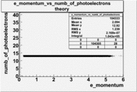
| + | The calculation of the number of photoelectrons emitted by electrons is shown below. | ||
| + | Electron mass <math>m_e = 0.000511GeV</math>, <math>n=1.00153</math> and <math>\beta=\frac{p}{E} = 1</math>, because mass of the electron is negligible and also <math>\frac{\alpha}{\hbar c}=370[ eV^{-1} cm^{-1}] </math><br><br> | ||
| + | The Hall B cherenkov detector is <math>\sim \; 0.7</math> m thick radiator. We assume the PMTs used to collect light have a constant quantum efficiency of 8% for photons with wavelength between 300 and 600 nm. | ||
| + | |||
| + | <math>\frac{dN}{dx} </math> <math>= 2 \pi \alpha z^2 [{\beta^2 n^2 (\lambda)} - 1]\int_{300nm}^{600nm} \frac{1}{\lambda^2} d\lambda \times (0.08)=</math> <br> | ||
| + | <math>= 2 \pi \alpha z^2 [{\beta^2 n^2 (\lambda)} - 1] (\frac {1}{\lambda})|_{600nm}^{300nm} \times (0.08) </math>=<br> | ||
| + | <math>= 2\times 3.14 \times \frac{1}{137} \times 1^2 \times [1.00153^2 - 1] \times \frac{1}{600} \times 0.08 [nm^{-1}] = </math> <br> | ||
| + | <math>= 19 \times 10^{-9} [nm^{-1}]</math> <br> | ||
| + | |||
| + | ;For the number of photoelectrons we have the following <br> | ||
| + | <math> N = 19 \times 10^{-9} \times 0.7 m [\frac{10^9}{m}] = 13.3 </math><br> | ||
| + | |||
| + | That means the number of photoelectrons should be about 13.<br> | ||
| + | |||
| + | Used file dst27095_05.B00 energy=5.7GeV and torus=2250(B>0). Target NH3<br> | ||
| + | |||
| + | [[Image:e_momentum_vs_numb_of_photoelectrons_27095_theory.gif|200px]] | ||
| + | |||
| + | ====Pions(<math>\pi^-</math>)==== | ||
| + | |||
| + | |||
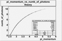
| + | The threshold energy for pions is ~2.5 GeV and for electrons 9 MeV. <br> | ||
| + | |||
| + | ;Example for <math>\pi^-</math> <br> | ||
| + | |||
| + | <math>m_{\pi^-}=139.57[\frac{MeV}{c^2}]</math>, momentum <math>p=mv=3 [\frac{GeV}{c}]</math> and n=1.00153<br> | ||
| + | |||
| + | where <math>\frac{\alpha}{\hbar c}=370[ eV^{-1} cm^{-1}] </math><br> | ||
| + | |||
| + | The Hall B cherenkov detector is <math>\sim \; 0.7</math> m thick radiator. We assume the PMTs used to collect light have a constant quantum efficiency of 8% for photons with wavelength between 300 and 600 nm. | ||
| + | |||
| + | <math>\frac{dN}{dx} = \frac{2 \pi \alpha z^2}{\lambda^2}[1-\frac{1}{\beta^2 n^2 (\lambda)}]=</math> <br> | ||
| + | <math>= 2 \pi \alpha z^2 [1-\frac{1}{\beta^2 n^2 (\lambda)}]\int_{300nm}^{600nm} \frac{1}{\lambda^2} d\lambda \times (0.08)=</math> <br> | ||
| + | <math>= 2 \pi \alpha z^2 [1-\frac{1}{\beta^2 n^2 (\lambda)}] (\frac {1}{\lambda})|_{600nm}^{300nm} \times (0.08) </math>=<br> | ||
| + | <math>= 2\times 3.14 \times \frac{1}{137} \times 1^2 \times [1-\frac{1}{0.998919^2 \times 1.00153^2}] \times \frac{1}{600} \times 0.08 [nm^{-1}] = </math> <br> | ||
| + | <math>= 5.465 \times 10^{-9} [nm^{-1}]</math> <br> | ||
| + | |||
| + | ;For the number of photons we have the following(for pions) <br> | ||
| + | <math> N = 5.465 \times 10^{-9} \times 0.7 m [\frac{10^9}{m}] = 3.8255 </math><br> | ||
| + | |||
| + | Used file dst27095_05.B00 energy=5.7GeV and torus=2250(B>0). Target NH3<br> | ||
| + | |||
| + | [[Image:pi_momentum_vs_numb_of_photons_27095_theory.gif|200px]] | ||
| + | |||
| + | ===CLAS Cherenkov signal=== | ||
| + | ====Electrons==== | ||
| + | |||
| + | The cherenkov signal measured in CLAS for particles identified as electrons by the tracking algorithm is shown below. There are two distributions present. One distribution is centered around 1.5 PEs and the second distribution is at 8 PEs when two gaussians and a Landau distribution are combined and fit to the spectrum. As we will show below, the first peak is due to the misidentification of a negative pion as an electron. | ||
| + | |||
| + | ;PE Fit equation | ||
| + | ;<math>N_{pe}= p_0 e^{-0.5 \left (\frac{x-p_1}{p_2} \right )^2} + p4\frac{1}{1-\left(\frac{x-p5}{p6}\right )} + p_6 e^{-0.5 \left (\frac{x-p_7}{p_8} \right )^2}</math> | ||
| + | |||
| + | [[Image:gaussian_fitting_function.pdf]] | ||
| + | |||
| + | C.Lanczos, SIAM Journal of Numerical Analysis B1 (1964), 86. | ||
| + | [[Image:C.Lanczos_SIAM_Journal_of_Numerical_Analysis_B1_1964_86.pdf]] | ||
| + | |||
| + | |||
| + | [http://ific.uv.es/informatica/manuales/root_v4.04/src/TFormula.cxx.html normalized fitting functions] | ||
| + | [http://wwwacs.gantep.edu.tr/guides/programming/root/htmldoc/TMath.html#TMath:Landau Landau and Landaun difference] | ||
| + | [http://support.adobe.com/devsup/devsup.nsf/docs/50023.htm for me] | ||
| + | |||
| + | //__[http://lcgapp.cern.ch/project/cls/work-packages/mathlibs/mathTable.html] [http://root.cern.ch/root/html/src/TMath.cxx.html#fsokrB] ____________________________________________________________________________ | ||
| + | Double_t TMath::Landau(Double_t x, Double_t mpv, Double_t sigma, Bool_t norm) | ||
| + | { | ||
| + | // The LANDAU function with mpv(most probable value) and sigma. | ||
| + | // This function has been adapted from the CERNLIB routine G110 denlan. | ||
| + | // If norm=kTRUE (default is kFALSE) the result is divided by sigma | ||
| + | static Double_t p1[5] = {0.4259894875,-0.1249762550, 0.03984243700, -0.006298287635, 0.001511162253}; | ||
| + | static Double_t q1[5] = {1.0 ,-0.3388260629, 0.09594393323, -0.01608042283, 0.003778942063}; | ||
| + | static Double_t p2[5] = {0.1788541609, 0.1173957403, 0.01488850518, -0.001394989411, 0.0001283617211}; | ||
| + | static Double_t q2[5] = {1.0 , 0.7428795082, 0.3153932961, 0.06694219548, 0.008790609714}; | ||
| + | static Double_t p3[5] = {0.1788544503, 0.09359161662,0.006325387654, 0.00006611667319,-0.000002031049101}; | ||
| + | static Double_t q3[5] = {1.0 , 0.6097809921, 0.2560616665, 0.04746722384, 0.006957301675}; | ||
| + | static Double_t p4[5] = {0.9874054407, 118.6723273, 849.2794360, -743.7792444, 427.0262186}; | ||
| + | static Double_t q4[5] = {1.0 , 106.8615961, 337.6496214, 2016.712389, 1597.063511}; | ||
| + | static Double_t p5[5] = {1.003675074, 167.5702434, 4789.711289, 21217.86767, -22324.94910}; | ||
| + | static Double_t q5[5] = {1.0 , 156.9424537, 3745.310488, 9834.698876, 66924.28357}; | ||
| + | static Double_t p6[5] = {1.000827619, 664.9143136, 62972.92665, 475554.6998, -5743609.109}; | ||
| + | static Double_t q6[5] = {1.0 , 651.4101098, 56974.73333, 165917.4725, -2815759.939}; | ||
| + | static Double_t a1[3] = {0.04166666667,-0.01996527778, 0.02709538966}; | ||
| + | static Double_t a2[2] = {-1.845568670,-4.284640743}; | ||
| + | if (sigma <= 0) return 0; | ||
| + | Double_t v = (x-mpv)/sigma; | ||
| + | Double_t u, ue, us, den; | ||
| + | if (v < -5.5) { | ||
| + | u = TMath::Exp(v+1.0); | ||
| + | if (u < 1e-10) return 0.0; | ||
| + | ue = TMath::Exp(-1/u); | ||
| + | us = TMath::Sqrt(u); | ||
| + | den = 0.3989422803*(ue/us)*(1+(a1[0]+(a1[1]+a1[2]*u)*u)*u); | ||
| + | } else if(v < -1) { | ||
| + | u = TMath::Exp(-v-1); | ||
| + | den = TMath::Exp(-u)*TMath::Sqrt(u)* | ||
| + | (p1[0]+(p1[1]+(p1[2]+(p1[3]+p1[4]*v)*v)*v)*v)/ | ||
| + | (q1[0]+(q1[1]+(q1[2]+(q1[3]+q1[4]*v)*v)*v)*v); | ||
| + | } else if(v < 1) { | ||
| + | den = (p2[0]+(p2[1]+(p2[2]+(p2[3]+p2[4]*v)*v)*v)*v)/ | ||
| + | (q2[0]+(q2[1]+(q2[2]+(q2[3]+q2[4]*v)*v)*v)*v); | ||
| + | } else if(v < 5) { | ||
| + | den = (p3[0]+(p3[1]+(p3[2]+(p3[3]+p3[4]*v)*v)*v)*v)/ | ||
| + | (q3[0]+(q3[1]+(q3[2]+(q3[3]+q3[4]*v)*v)*v)*v); | ||
| + | } else if(v < 12) { | ||
| + | u = 1/v; | ||
| + | den = u*u*(p4[0]+(p4[1]+(p4[2]+(p4[3]+p4[4]*u)*u)*u)*u)/ | ||
| + | (q4[0]+(q4[1]+(q4[2]+(q4[3]+q4[4]*u)*u)*u)*u); | ||
| + | } else if(v < 50) { | ||
| + | u = 1/v; | ||
| + | den = u*u*(p5[0]+(p5[1]+(p5[2]+(p5[3]+p5[4]*u)*u)*u)*u)/ | ||
| + | (q5[0]+(q5[1]+(q5[2]+(q5[3]+q5[4]*u)*u)*u)*u); | ||
| + | } else if(v < 300) { | ||
| + | u = 1/v; | ||
| + | den = u*u*(p6[0]+(p6[1]+(p6[2]+(p6[3]+p6[4]*u)*u)*u)*u)/ | ||
| + | (q6[0]+(q6[1]+(q6[2]+(q6[3]+q6[4]*u)*u)*u)*u); | ||
| + | } else { | ||
| + | u = 1/(v-v*TMath::Log(v)/(v+1)); | ||
| + | den = u*u*(1+(a2[0]+a2[1]*u)*u); | ||
| + | } | ||
| + | if (!norm) return den; | ||
| + | return den/sigma; | ||
| + | }<br> | ||
| + | |||
| + | Fitting the Histograms<br> | ||
| + | |||
| + | root [13] e_numb_of_photoelectrons->Draw(); <br> | ||
| + | root [2] g3= new TF1("g3","gaus(0)+landau(3)+gaus(6)",0,20); <br> | ||
| + | |||
| + | To get fit parameters for g3 we should fit individually each of them(gaus(0),landau(3),gaus(6))<br> | ||
| + | |||
| + | root [3] g3->SetParameters(2.3e3,8,8.1,8.6e+3,8.6e-1,1.6,8.6e+3,8.6e-1,1.6,8.6e3)<br> | ||
| + | root [11] e_numb_of_photoelectrons->Fit("g3","R+"); | ||
| + | |||
| + | ;e_Momentum_vs_Number_of_Photoelectrons | ||
| + | |||
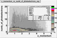
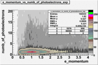
| + | The flag cut applied on the number of photoelectrons means that in CLAS detector instead of 5 superlayers were used 6 of them in track fit. As one can see from the histograms of the Number of photoelectrons, the cut on flag does not have effect on the peak around 1.5phe and decreases the number of entries by 37.17 %. The peak is due to a high energy pions(>2.5GeV), which have enough momentum to emit Cherenkov light and also because of the bad collection of light, there are a particular polar and azimuthal combination of angles where The Cherencov Detector cannot receive emitted light. .<br> | ||
| + | |||
| + | ;Number of photoelectrons | ||
| + | |||
| + | |||
| + | {|border="2" colspan = "4" | ||
| + | !Data|||||| | ||
| + | |- | ||
| + | | ||[[Image:e_number_of_photoelectrons_27095_1.gif|200px]] | ||
| + | || [[Image:e_number_of_photoelectrons_27095_fits.gif|200px]] | ||
| + | |- | ||
| + | | ||[[Image:e_number_of_photoelectrons_27095_flag_10_1.gif|200px]] | ||
| + | || [[Image:e_number_of_photoelectrons_27095_flag_10_fit_with_cut.gif|200px]] | ||
| + | |}<br> | ||
| + | |||
| + | Table: Cherenkov fit values | ||
| + | |||
| + | {|border="2" colspan = "4" | ||
| + | !Distributions||amplitude|| mean || width ||amplitude|| mean || width | ||
| + | |- | ||
| + | | || colspan="3" align="center"| without cuts|| colspan="3" align="center"| with cut(flag>10) | ||
| + | |- | ||
| + | | gauss(0)|| p0=2144+/-44.0 || p1=5.342+/-0.343 || p2=7.761+/-0.188 || p0=1580+/-8.1 || p1=3.75+/-0.06 || p2=8.486+/-0.042 | ||
| + | |- | ||
| + | | landau(3)|| p3=4.349e+04+/-2894 || p4=1.049+/-0.026 || p5=0.2197+/-0.0257 || p3=8600+/-3648.7 || p4=-3.861+/-1.414 || p5=-4.88+/-1.41 | ||
| + | |- | ||
| + | | gauss(6)|| p6=4960+/-270.6 || p7=0.7345+/-0.0983 || p8=0.8885+/-0.0594 || p6=6219+/-54.2 || p7=1.088+/-0.006 || p8=0.6037+/-0.0052 | ||
| + | |}<br> | ||
| + | |||
| + | |||
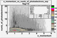
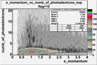
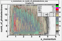
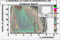
| + | When flag cut(flag>10 cut means that 6 superlayers were used in track fit) was applied the number of entries decreased by 37.17 % and the mean value for the number of photoelectrons is about 7-8. After 5<nphe<15 cut, the number of entries decreased by 66.63 %.The mean value of the nphe is ~9 which agrees with theory(mean value ~13).<br> | ||
| + | |||
| + | |||
| + | {|border="2" colspan = "4" | ||
| + | !Experiment||B>0||without cuts||flag>10||5<nphe<15||5<nphe<15 and flag>10 | ||
| + | |- | ||
| + | | || ||[[Image:e_momentum_vs_numb_of_photoelectrons_27095_exp_without_cuts_1.gif|200px]] | ||
| + | [[Image:e_momentum_vs_numb_of_photoelectrons_27095_exp_without_cuts_2.gif|200px]] | ||
| + | [[Image:e_momentum_vs_numb_of_photoelectrons_27095_exp_without_cuts_3.gif|200px]] | ||
| + | || [[Image:e_momentum_vs_numb_of_photoelectrons_27095_exp_with_cuts_flag_10_1.gif|200px]] | ||
| + | [[Image:e_momentum_vs_numb_of_photoelectrons_27095_exp_with_cuts_flag_10_2.gif|200px]] | ||
| + | [[Image:e_momentum_vs_numb_of_photoelectrons_27095_exp_with_cuts_flag_10_3.gif|200px]] | ||
| + | || [[Image:e_momentum_vs_numb_of_photoelectrons_27095_exp_with_cuts_?_nphe_?.gif|200px]] | ||
| + | ||[[Image:e_momentum_vs_numb_of_photoelectrons_27095_exp_with_cuts_5_nphe_15_flag_10.gif|200px]] | ||
| + | |} | ||
| + | |||
| + | ====Pions(<math>\pi^-</math>)==== | ||
| + | |||
| + | ;<math>\pi^-</math>_Momentum_vs_Number_of_Photons | ||
| + | |||
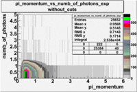
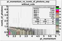
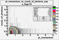
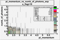
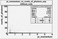
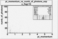
| + | After e_flag>10 cut, the number of entries decreased by 30.45 % and the mean value for the number of photons is ~9 | ||
| + | |||
| + | |||
| + | {|border="2" colspan = "4" | ||
| + | !Experiment||B>0||without cuts||e_flag>10||0<e_nphe<5||0<nphe<5 and e_flag>10 | ||
| + | |- | ||
| + | | || ||[[Image:pi_momentum_vs_numb_of_photoelectrons_27095_exp_without_cuts_1_1.gif|200px]] | ||
| + | [[Image:pi_momentum_vs_numb_of_photoelectrons_27095_exp_without_cuts_2_1.gif|200px]] | ||
| + | [[Image:pi_momentum_vs_numb_of_photoelectrons_27095_exp_without_cuts_3_1.gif|200px]] | ||
| + | || [[Image:pi_momentum_vs_numb_of_photoelectrons_27095_exp_with_cuts_flag_10_1_1.gif|200px]] | ||
| + | [[Image:pi_momentum_vs_numb_of_photoelectrons_27095_exp_with_cuts_flag_10_2_1.gif|200px]] | ||
| + | [[Image:pi_momentum_vs_numb_of_photoelectrons_27095_exp_with_cuts_flag_10_3_1.gif|200px]] | ||
| + | || [[Image:pi_momentum_vs_numb_of_photoelectrons_27095_exp_with_cuts_?_nphe_?.gif|200px]] | ||
| + | ||[[Image:pi_momentum_vs_numb_of_photoelectrons_27095_exp_with_cuts_0_nphe_5_flag_10.gif|200px]] | ||
| + | |} | ||
Revision as of 14:39, 15 January 2009
15-1-09
Cherenkov
Cherenkov Theory
When the velocity of a charged particle is greater than the local phase velocity of light or when it enters a medium with different optical properties the charged particle will emit photons. The Cherenkov light is emitted under a constant angle - the angle of Cherenkov radiation relative to the particle's direction. It can be shown geometrically that the cosine of the Cherenkov radiation angle is anti-proportional to the velocity of the charged particle
where is the particle's velocity and n - index of refraction of the medium.The charged particle in time t travels distance, while the electromagnetic waves - . For a medium with given index of refraction n there is a threshold velocity , below no radiation can take place. This process may be used to observe the passage of charged particles in a detector which can measure the produced photons.
The number of photons produced per unit path length of a particle with charge ze and per unit energy interval of the photons is proportional to the sine of the Cherenkov angle[1]
after deriving the Taylor expansion of our function and considering only the first two terms, we get
The gas used in the CLAS Cerenkov counter is perfluorobutane with index of refraction equal to 1.00153.
Electrons
The calculation of the number of photoelectrons emitted by electrons is shown below.
Electron mass , and , because mass of the electron is negligible and also
The Hall B cherenkov detector is m thick radiator. We assume the PMTs used to collect light have a constant quantum efficiency of 8% for photons with wavelength between 300 and 600 nm.
=
- For the number of photoelectrons we have the following
That means the number of photoelectrons should be about 13.
Used file dst27095_05.B00 energy=5.7GeV and torus=2250(B>0). Target NH3
Pions()
The threshold energy for pions is ~2.5 GeV and for electrons 9 MeV.
- Example for
, momentum and n=1.00153
where
The Hall B cherenkov detector is m thick radiator. We assume the PMTs used to collect light have a constant quantum efficiency of 8% for photons with wavelength between 300 and 600 nm.
=
- For the number of photons we have the following(for pions)
Used file dst27095_05.B00 energy=5.7GeV and torus=2250(B>0). Target NH3
CLAS Cherenkov signal
Electrons
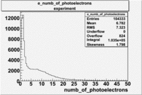
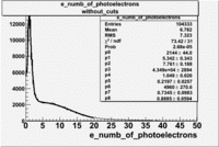
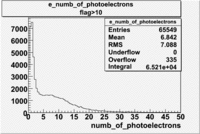
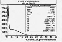
The cherenkov signal measured in CLAS for particles identified as electrons by the tracking algorithm is shown below. There are two distributions present. One distribution is centered around 1.5 PEs and the second distribution is at 8 PEs when two gaussians and a Landau distribution are combined and fit to the spectrum. As we will show below, the first peak is due to the misidentification of a negative pion as an electron.
- PE Fit equation
File:Gaussian fitting function.pdf
C.Lanczos, SIAM Journal of Numerical Analysis B1 (1964), 86.
File:C.Lanczos SIAM Journal of Numerical Analysis B1 1964 86.pdf
normalized fitting functions
Landau and Landaun difference
for me
//__[2] [3] ____________________________________________________________________________
Double_t TMath::Landau(Double_t x, Double_t mpv, Double_t sigma, Bool_t norm)
{
  // The LANDAU function with mpv(most probable value) and sigma.
  // This function has been adapted from the CERNLIB routine G110 denlan.
  // If norm=kTRUE (default is kFALSE) the result is divided by sigma
  static Double_t p1[5] = {0.4259894875,-0.1249762550, 0.03984243700, -0.006298287635,   0.001511162253};
  static Double_t q1[5] = {1.0         ,-0.3388260629, 0.09594393323, -0.01608042283,    0.003778942063};
  static Double_t p2[5] = {0.1788541609, 0.1173957403, 0.01488850518, -0.001394989411,   0.0001283617211};
  static Double_t q2[5] = {1.0         , 0.7428795082, 0.3153932961,   0.06694219548,    0.008790609714};
  static Double_t p3[5] = {0.1788544503, 0.09359161662,0.006325387654, 0.00006611667319,-0.000002031049101};
  static Double_t q3[5] = {1.0         , 0.6097809921, 0.2560616665,   0.04746722384,    0.006957301675};
  static Double_t p4[5] = {0.9874054407, 118.6723273,  849.2794360,   -743.7792444,      427.0262186};
  static Double_t q4[5] = {1.0         , 106.8615961,  337.6496214,    2016.712389,      1597.063511};
  static Double_t p5[5] = {1.003675074,  167.5702434,  4789.711289,    21217.86767,     -22324.94910};
  static Double_t q5[5] = {1.0         , 156.9424537,  3745.310488,    9834.698876,      66924.28357};
  static Double_t p6[5] = {1.000827619,  664.9143136,  62972.92665,    475554.6998,     -5743609.109};
  static Double_t q6[5] = {1.0         , 651.4101098,  56974.73333,    165917.4725,     -2815759.939};
  static Double_t a1[3] = {0.04166666667,-0.01996527778, 0.02709538966};
  static Double_t a2[2] = {-1.845568670,-4.284640743};
  if (sigma <= 0) return 0;
  Double_t v = (x-mpv)/sigma;
  Double_t u, ue, us, den;
  if (v < -5.5) {
     u   = TMath::Exp(v+1.0);
     if (u < 1e-10) return 0.0;
     ue  = TMath::Exp(-1/u);
     us  = TMath::Sqrt(u);
     den = 0.3989422803*(ue/us)*(1+(a1[0]+(a1[1]+a1[2]*u)*u)*u);
  } else if(v < -1) {
     u   = TMath::Exp(-v-1);
     den = TMath::Exp(-u)*TMath::Sqrt(u)*
            (p1[0]+(p1[1]+(p1[2]+(p1[3]+p1[4]*v)*v)*v)*v)/
            (q1[0]+(q1[1]+(q1[2]+(q1[3]+q1[4]*v)*v)*v)*v);
  } else if(v < 1) {
     den = (p2[0]+(p2[1]+(p2[2]+(p2[3]+p2[4]*v)*v)*v)*v)/
           (q2[0]+(q2[1]+(q2[2]+(q2[3]+q2[4]*v)*v)*v)*v);
  } else if(v < 5) {
     den = (p3[0]+(p3[1]+(p3[2]+(p3[3]+p3[4]*v)*v)*v)*v)/
           (q3[0]+(q3[1]+(q3[2]+(q3[3]+q3[4]*v)*v)*v)*v);
  } else if(v < 12) {
     u   = 1/v;
     den = u*u*(p4[0]+(p4[1]+(p4[2]+(p4[3]+p4[4]*u)*u)*u)*u)/
               (q4[0]+(q4[1]+(q4[2]+(q4[3]+q4[4]*u)*u)*u)*u);
  } else if(v < 50) {
     u   = 1/v;
     den = u*u*(p5[0]+(p5[1]+(p5[2]+(p5[3]+p5[4]*u)*u)*u)*u)/
               (q5[0]+(q5[1]+(q5[2]+(q5[3]+q5[4]*u)*u)*u)*u);
  } else if(v < 300) {
     u   = 1/v;
     den = u*u*(p6[0]+(p6[1]+(p6[2]+(p6[3]+p6[4]*u)*u)*u)*u)/
               (q6[0]+(q6[1]+(q6[2]+(q6[3]+q6[4]*u)*u)*u)*u);
  } else {
     u   = 1/(v-v*TMath::Log(v)/(v+1));
     den = u*u*(1+(a2[0]+a2[1]*u)*u);
  }
  if (!norm) return den;
  return den/sigma;
}
Fitting the Histograms
root [13] e_numb_of_photoelectrons->Draw();

root [2] g3= new TF1("g3","gaus(0)+landau(3)+gaus(6)",0,20);
To get fit parameters for g3 we should fit individually each of them(gaus(0),landau(3),gaus(6))
root [3] g3->SetParameters(2.3e3,8,8.1,8.6e+3,8.6e-1,1.6,8.6e+3,8.6e-1,1.6,8.6e3)

root [11] e_numb_of_photoelectrons->Fit("g3","R+");
- e_Momentum_vs_Number_of_Photoelectrons
The flag cut applied on the number of photoelectrons means that in CLAS detector instead of 5 superlayers were used 6 of them in track fit. As one can see from the histograms of the Number of photoelectrons, the cut on flag does not have effect on the peak around 1.5phe and decreases the number of entries by 37.17 %. The peak is due to a high energy pions(>2.5GeV), which have enough momentum to emit Cherenkov light and also because of the bad collection of light, there are a particular polar and azimuthal combination of angles where The Cherencov Detector cannot receive emitted light. .
- Number of photoelectrons
| Data | |||
|---|---|---|---|
|
| ||
|
|
Table: Cherenkov fit values
| Distributions | amplitude | mean | width | amplitude | mean | width |
|---|---|---|---|---|---|---|
| without cuts | with cut(flag>10) | |||||
| gauss(0) | p0=2144+/-44.0 | p1=5.342+/-0.343 | p2=7.761+/-0.188 | p0=1580+/-8.1 | p1=3.75+/-0.06 | p2=8.486+/-0.042 |
| landau(3) | p3=4.349e+04+/-2894 | p4=1.049+/-0.026 | p5=0.2197+/-0.0257 | p3=8600+/-3648.7 | p4=-3.861+/-1.414 | p5=-4.88+/-1.41 |
| gauss(6) | p6=4960+/-270.6 | p7=0.7345+/-0.0983 | p8=0.8885+/-0.0594 | p6=6219+/-54.2 | p7=1.088+/-0.006 | p8=0.6037+/-0.0052 |
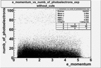
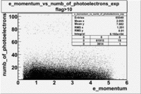
When flag cut(flag>10 cut means that 6 superlayers were used in track fit) was applied the number of entries decreased by 37.17 % and the mean value for the number of photoelectrons is about 7-8. After 5<nphe<15 cut, the number of entries decreased by 66.63 %.The mean value of the nphe is ~9 which agrees with theory(mean value ~13).
| Experiment | B>0 | without cuts | flag>10 | 5<nphe<15 | 5<nphe<15 and flag>10 |
|---|---|---|---|---|---|
|
|
|
|
Pions()
- _Momentum_vs_Number_of_Photons
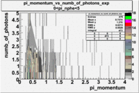
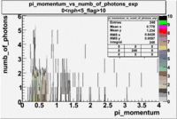
After e_flag>10 cut, the number of entries decreased by 30.45 % and the mean value for the number of photons is ~9
| Experiment | B>0 | without cuts | e_flag>10 | 0<e_nphe<5 | 0<nphe<5 and e_flag>10 |
|---|---|---|---|---|---|
|
|
|
|
