Detector Geometry
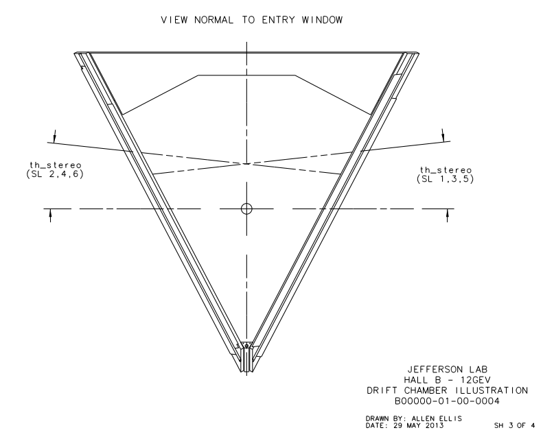
Examining the geometry of the Drift Chamber, we can see that the detector is similar to a hexagonal pyramid in shape.
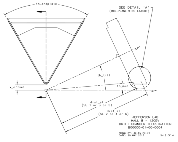
Figure 1: A graphical rendering of a drift chamber sector.
From the geometry it is given that xdist, the distance between the line of intersection of the two end-plate planes and the target position, is equal to 8.298 cm and th_min, the angle from the target vertex to the the same line, is 4.694 degrees. Using this knowledge we can simulate this situation by having the end-plate planes intersect at the beam line axis. This action in effect would grant the sector to measure angles below ~5 degrees, which we can account for by limiting angles theta within the accepted detector range. The quantity dist2tgt, the distance from the target to the first guard wire plane along the normal of said plane, is given as 228.078 cm. Using the previous understanding of the distances between planes within a Superlayer:
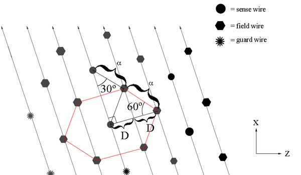
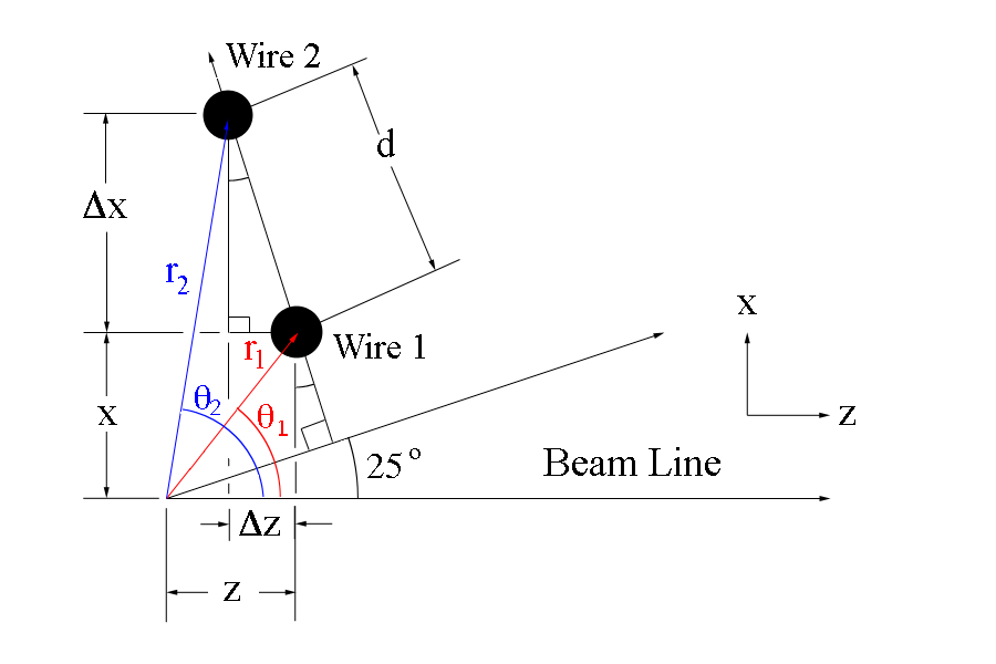
Figure 2: A graphical rendering of a drift chamber wire spacing.
We know that the seperation between levels is a constant D=.3861 cm, and that sensor layer 1 is 3 layers deep.
This gives us the distance to level 1 from the vertex (0,0,0) as 228.078 cm+3(0.3861) cm=229.2363 cm in the normal direction from the wire plane to the target. Using the fact that the wire planes are at 25 degrees to the beam line normal, we can approximate sector one as triangle that intersects with a line perpendicular to the beam line at the vertex position of (0,0,0) along the bisector of the triangle. This then by geometry shown in the figure below implies the distance traveling along the beam line would intersect the theoretical extension of the sector at z= 2.53 m. While this is beyond the physical constructs of the experimental design, we do this mathematical simplicity. This again is acceptable in that angles beyond the physical limitations of 40 degrees will not be simulated. From the geometry of a hexagonal pyramid, we can see that the quantity h should be
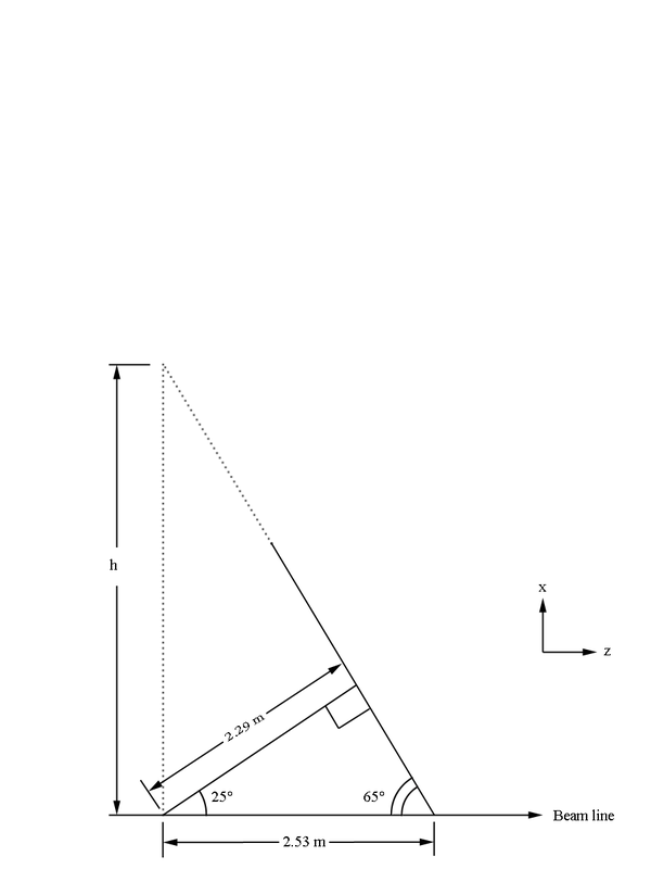
Figure 3: A graphical rendering of a drift chamber wire spacing from the side.
[math]h=\frac{2.292363\ m}{sin(25^{\circ})}[/math]
[math]h=5.42\ m[/math]
Examining the geometry of a hexagonal of h=[math]\sqrt{3}\approx1.732[/math] whose coordinates are easy to calculate:
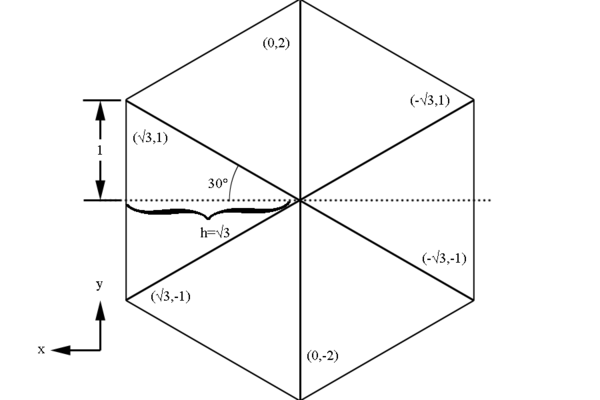
Figure 4: A graphical rendering of a drift chamber geometry.
We can scale this hexagon by a factor of 3.13 to find the base of the hexagonal pyramid simulating the drift chamber geometry.
sector1=Graphics3D[{Red,Opacity[.8],Polygon[{{0,0,2.53},{3.13\[Sqrt]3,3.13,0},{3.13\[Sqrt]3,-3.13,0}}]},BoxStyle->Dashing[{0.02,0.02}],Axes->True,AxesLabel->{"x","y","z"},Ticks->None,AxesStyle->Thickness[0.01]];
sector2=Graphics3D[{GrayLevel[0.5],Opacity[.2],Polygon[{{0,0,2.53},{3.13\[Sqrt]3,-3.13,0},{0,-2*3.13,0}}]},BoxStyle->Dashing[{0.02,0.02}],Axes->True,AxesLabel->{"x","y","z"},Ticks->None,AxesStyle->Thickness[0.01]];
sector3=Graphics3D[{GrayLevel[0.5],Opacity[.2],Polygon[{{0,0,2.53},{0,-2*3.13,0},{-3.13\[Sqrt]3,-3.13,0}}]},BoxStyle->Dashing[{0.02,0.02}],Axes->True,AxesLabel->{"x","y","z"},Ticks->None,AxesStyle->Thickness[0.01]];
sector4=Graphics3D[{GrayLevel[0.5],Opacity[.2],Polygon[{{0,0,2.53},{-3.13\[Sqrt]3,-3.13,0},{-3.13\[Sqrt]3,3.13,0}}]},BoxStyle->Dashing[{0.02,0.02}],Axes->True,AxesLabel->{"x","y","z"},Ticks->None,AxesStyle->Thickness[0.01]];
sector5=Graphics3D[{GrayLevel[0.5],Opacity[.2],Polygon[{{0,0,2.53},{-3.13\[Sqrt]3,3.13,0},{0,2*3.13,0}}]},BoxStyle->Dashing[{0.02,0.02}],Axes->True,AxesLabel->{"x","y","z"},Ticks->None,AxesStyle->Thickness[0.01]];
sector6=Graphics3D[{GrayLevel[0.5],Opacity[.2],Polygon[{{0,0,2.53},{0,2*3.13,0},{3.13\[Sqrt]3,3.13,0}}]},BoxStyle->Dashing[{0.02,0.02}],Axes->True,AxesLabel->{"x","y","z"},Ticks->None,AxesStyle->Thickness[0.01]];
Bisector0Sector1=Graphics3D[Line[{{0,0,2.53},{3.13\[Sqrt]3,0,0}}]];
Bisector0perpSector1=Graphics3D[Line[{{0,0,0},{3.13\[Sqrt]3,0,0}}]];
RightAngleVertical=Graphics3D[Line[{{.25,0,.25},{.25,0,0}}]];
RightAngleHorizontal=Graphics3D[Line[{{.25,0,.25},{0,0,.25}}]];
Bisector0Cone=Graphics3D[Line[{{3.13\[Sqrt]3,0,0},{3.13\[Sqrt]3,0,2.53}}]];
Bisector0perpCone=Graphics3D[Line[{{0,0,2.53},{3.13\[Sqrt]3,0,2.53}}]];
RightAngleVertical2=Graphics3D[Line[{{3.13\[Sqrt]3-.25,0,2.53-.25},{3.13\[Sqrt]3-.25,0,2.53}}]];
RightAngleHorizontal2=Graphics3D[Line[{{3.13\[Sqrt]3-.25,0,2.53-.25},{3.13\[Sqrt]3,0,2.53-.25}}]];
BeamLine=Graphics3D[Arrow[{{0,0,-.5},{0,0,2.79}}]];
PhiCone=Graphics3D[{Blue,Opacity[.3],Cone[{{0,0,2.53},{0,0,0}},3.13\[Sqrt]3]},BoxStyle->Dashing[{0.02,0.02}],Axes->True,AxesLabel->{"x","y","z"},Ticks->None,AxesStyle->Thickness[0.01]];
Viewing the simulation,
Show[sector1,sector2,sector3,sector4,sector5,sector6,PhiCone,BeamLine,Bisector0Sector1,Bisector0perpSector1,Bisector0Cone,Bisector0perpCone,RightAngleVertical,RightAngleHorizontal,RightAngleVertical2,RightAngleHorizontal2]
When the scattering angle theta, which is measured with respect to the beam line, is held constant and rotated through 360 degrees in phi, a cone is created. Using Mathematica, we can produce a 3D rendering of how the sectors for Level 1 would have to interact with a steady angle theta with respect to the beam line, as angle phi is rotated through 360 degrees.
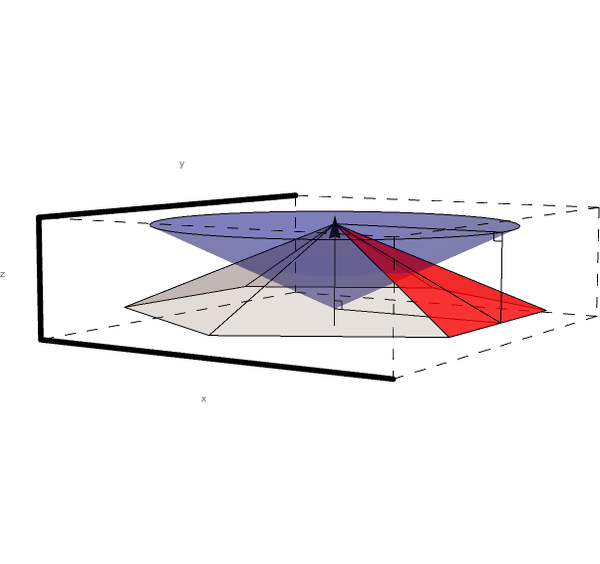
Figure 5: A cone of constant Theta with varying Phi.
Conic Sections
Looking just at sector 1, we can see that the intersection of level 1 and the cone of constant angle theta forms a conic section.
Show[sector1,PhiCone,BeamLine,Bisector0Sector1,Bisector0perpSector1,Bisector0Cone,Bisector0perpCone,RightAngleVertical,RightAngleHorizontal,RightAngleVertical2,RightAngleHorizontal2]
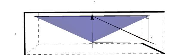
Figure 5: A cone of constant Theta with varying Phi.
Without loss of generalization, we can extend the triangle to an infinite plane to aid in viewing the conic section. Again, this falls outside of the experimental design range, but simulations would not occur in this forbidden zone.
sector1plane =
  Graphics3D[{Red, Opacity[.8],
    InfinitePlane[{{0, 0, 2.53}, {3.13 \[Sqrt]3, .617,
       0}, {3.13 \[Sqrt]3, -3.13, 0}}]},
   BoxStyle -> Dashing[{0.02, 0.02}], Axes -> True,
   AxesLabel -> {"x", "y", "z"}, Ticks -> None,
   AxesStyle -> Thickness[0.01]];

Show[sector1plane, PhiCone, BeamLine, Bisector0Sector1, \
Bisector0perpSector1, Bisector0Cone, Bisector0perpCone, \
RightAngleVertical, RightAngleHorizontal, RightAngleVertical2, \
RightAngleHorizontal2]
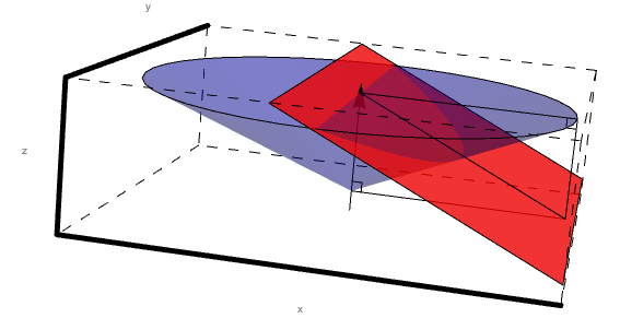
Figure 5: A cone of constant Theta with varying Phi.
Following the rules of conic sections we know that the eccentricity of the conic is given by:
[math]e=\frac{\sin \beta}{\sin\alpha}[/math]
where β is the angle between the plane and the horizontal and α is the angle between the cone's base and the horizontal.
Examining the different conic sections possible we know that:
Circular Conic Section
If the conic is an circle, e=0. This implies
[math]e=\frac{\sin (\beta)}{\sin (\alpha)}=\frac{\sin (25^{\circ})}{\sin (90-\theta)}=0[/math]
Using the relation
[math]sin(90^{\circ}-\theta)=cos(\theta)[/math]
[math]\frac{sin (25^{\circ})}{0}=cos( \theta) =\infty[/math]
The sector angle will never be perpendicular to the plane of the light cone, so this is not a physical possibility.
Elliptic Conic Section
If the conic is an ellipse, 0<e<1. This implies
[math]e=\frac{\sin \beta}{\sin \alpha}=\frac{\sin\ (25^{\circ})}{\sin (90^{\circ}-\theta)}[/math]
[math]\frac{sin (25^{\circ})}{cos (\theta)}=e[/math]
since e must be less than 1, this sets the limit of theta at less than 65 degrees. Since the limit of [math]\theta=0[/math], this implies the minimum eccentricity will be [math]e\approx .4291[/math]
This implies that the shape made on the the plane of the sector is an ellipse for angles
[math] 0\lt \theta\lt 65^{\circ}[/math]
Determining ellipse components
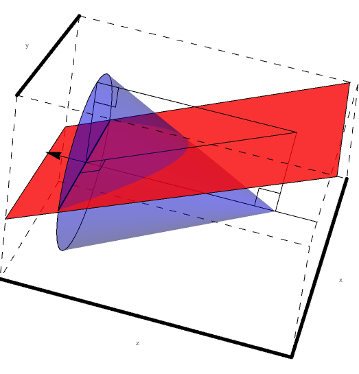
Figure 5: A cone of constant Theta with varying Phi.
Here we must take note of the fact that the center of the cone and the center of the ellipse do not coincide as can be shown visually by extending the cone length.
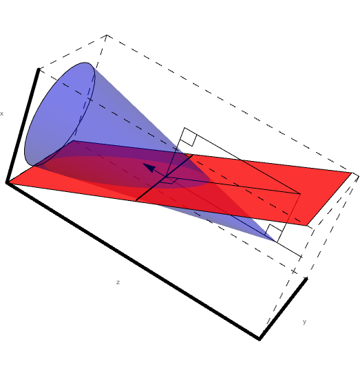
Figure 5: A cone of constant Theta with varying Phi.
Here we will make use of Dandelin spheres to help determine the ellipse components with reference to the cone created at a constant theta. The basic construction of using Dandelin spheres is that within the cone, there are two spheres which are tangent to the plane as well as tangent to the cone as shown below in the xz plane. The Dandelin method picks an arbitrary point,P, on the intersection of the cone and the ellipse's plane. Drawing a line from the cone vertex through the point P, the directrix lines are intersected as shown below at D1 and D2. From the geometry as shown in the xz plane, it is shown that the line segments F1P=D1P and F2P=D2P since they share a common line segment, all three angles, and both have a the respective Dandelin radius as parts of the triangles they form.
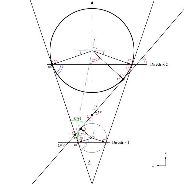
Figure 5: A cone of constant Theta with varying Phi.
We can use the law of sines to find a portion of the ellipse
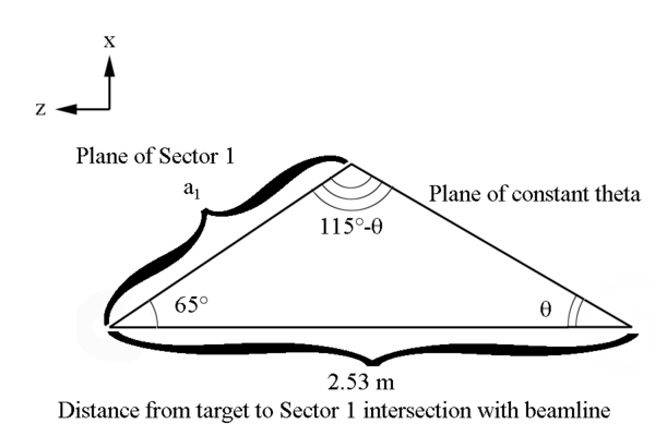
Figure 5: A cone of constant Theta with varying Phi.
[math]\frac{2.53\ m}{sin(115^{\circ}-\theta)}=\frac{a_1}{sin(\theta)}[/math]
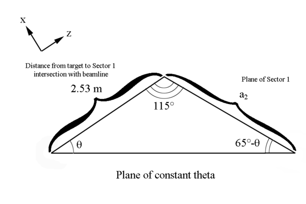
Figure 5: A cone of constant Theta with varying Phi.
[math]\frac{a}{sin(A)}=\frac{b}{sin(B)}[/math]
[math]\frac{2.53\ m}{sin(65^{\circ}-\theta)}=\frac{a_2}{sin(\theta)}[/math]
Since these lines meet at the intersection of each other, and they both originate at the vertex positions for the ellipse, we can state that the semi major axis is:
[math]2a\equiv a_1+a_2[/math]
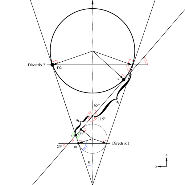
Figure 5: A cone of constant Theta with varying Phi.
Using the fact that half the semi-major axis will give use the center of the ellipse
[math]a=\frac{a_1+a_2}{2}[/math]
[math]a=\frac{2.53sin(\theta)}{2}\left (\frac{sin(115^{\circ}-\theta)+sin(65^{\circ}-\theta)}{sin(115^{\circ}-\theta)sin(65^{\circ}-\theta)}\right )[/math]
[math]a=\frac{2.53sin(\theta)}{2}\left (sin(115^{\circ}-\theta)+sin(65^{\circ}-\theta)\right ) csc(115^{\circ}-\theta)csc(65^{\circ}-\theta)[/math]
| [math]a=\frac{2.53sin(\theta)}{2}\left (csc(65^{\circ}-\theta)+csc(115^{\circ}-\theta) \right )[/math]
|
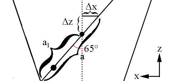
Figure 5: A cone of constant Theta with varying Phi.
Earlier, using the law of sines it was found:
[math]\frac{2.53\ m}{sin(115^{\circ}-\theta)}=\frac{a_1}{sin(\theta)}[/math]
[math]\frac{2.53\ m \cdot sin(\theta)}{sin(115^{\circ}-\theta)}=a_1[/math]
Taking the difference
[math]\Delta a=a-a_1=\frac{a_1+a_2}{2}-a_1=\frac{a_2-a_1}{2}[/math]
| [math]\Delta a=\frac{2.53sin(\theta)}{2}\left (csc(65^{\circ}-\theta)-csc(115^{\circ}-\theta) \right )[/math]
|
[math]\Delta z=\Delta a \cdot cos(65^{\circ})[/math]
[math]\Delta x=\Delta a \cdot sin(65^{\circ})[/math]
Since the vertex position is at (0,0,0) this shows the center of the ellipse to be at
[math]c_{ellipse} \equiv (-\Delta a sin(65^{\circ}), 0,z+\Delta z)[/math]
[math]c_{ellipse} \equiv (-\Delta a sin(65^{\circ}), 0,2.53+\Delta z)[/math]
The sum of the distance from both focal points to a point on the surface of the ellipse is a constant

Figure 5: A cone of constant Theta with varying Phi.
A property of an ellipse is that the distance from the center of the ellipse to a focal point is given by
[math]f=ae=\left (\frac{a_1+a_2}{2}\right ) \left ( \frac{sin(25^{\circ})}{cos(\theta)}\right )[/math]
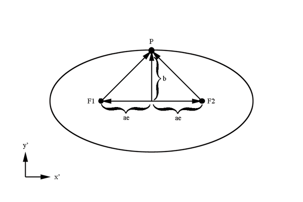
Figure 5: A cone of constant Theta with varying Phi.
[math]2ae+2b=2a\Rightarrow b=a(1-e)[/math]
[math]b=\left (\frac{a_1+a_2}{2}\right ) \left (1-\frac{sin(25^{\circ})}{cos(\theta)}\right )[/math]
[math]b=\frac{2.53sin(\theta)}{2}\left (\frac{sin(115^{\circ}-\theta)+sin(65^{\circ}-\theta)}{sin(115^{\circ}-\theta)sin(65^{\circ}-\theta)}\right ) \left (1-\frac{sin(25^{\circ})}{cos(\theta)}\right )[/math]
Additionally, using the fact that the distance from the center to a focal point is ae
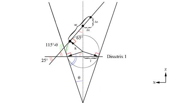
Figure 5: A cone of constant Theta with varying Phi.
[math]R_{Lower\ Dandelin}=(ae-\Delta a) tan(65^{\circ})[/math]
[math]r_{D1}=R_{Lower\ Dandelin}sec(\theta)=(ae-\Delta a) tan(65^{\circ})cos(\theta)[/math]
By symmetry,
[math]R_{Upper\ Dandelin}=(ae+\Delta a) tan(65^{\circ})[/math]
[math]r_{D2}=R_{Lower\ Dandelin}sec(\theta)=(ae+\Delta a) tan(65^{\circ})cos(\theta)[/math]
Determining Elliptical Equation
As found earlier
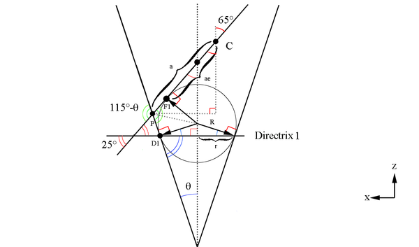
Figure 5: A cone of constant Theta with varying Phi.
[math]CP_x=a\ sin(65^{\circ})[/math]
[math]CP_z=a\ cos(65^{\circ})[/math]
Given the center point coordinates found earlier:
[math]c \equiv (-\Delta x, 0,z+\Delta z)[/math]
[math]c \equiv (-\Delta a\ sin(65^{\circ}), 0,z+\Delta a\ cos(65^{\circ}))[/math]
This gives the location of P([math]\phi=0[/math]) at
[math]P(\phi=0) \equiv (-\Delta a\ sin(65^{\circ})+a\ sin((65^{\circ}), 0,z+\Delta a\ cos(65^{\circ})-a\ cos(65^{\circ}))[/math]
[math]P(\phi=0) \equiv (-\frac{a_2-a_1}{2} sin(65^{\circ})+\frac{a_1+a_2}{2} sin((65^{\circ}), 0,2.53+\frac{a_2-a_1}{2} cos(65^{\circ})-\frac{a_1+a_2}{2} cos(65^{\circ}))[/math]
The height in z can be viewed as a linear function of x and expressed in slope intercept form for a plane:
[math]z_{Plane\ of\ sector}=m_{plane}x+b_{plane}[/math]
where
[math]m_{plane}=\frac{\Delta z}{\Delta x}=\frac{a\ cos(65^{\circ})}{-a\ sin(65^{\circ})}=-cot(65^{\circ})[/math]
[math]b_{plane}\equiv (0,0,2.53)[/math]
The D1 and D2 components can be obtained by finding the x and y components of the two directrix circles, which will be a function of their respective radii and the angle phi around the z axis.
[math]x_{Lower\ Directrix}^2+y_{Lower\ Directrix}^2=r_{Lower\ Directrix}^2\equiv r_{Lower\ Directrix}^2 cos^2(\phi)+r_{Lower\ Directrix}^2 sin^2(\phi)[/math]
Solving for the cartesian components,
[math]x_{Lower\ Directrix}=r_{Lower\ Directrix}\ cos(\phi)\qquad \qquad \qquad y_{Lower\ Directrix}=r_{Lower\ Directrix}\ sin(\phi)[/math]
Similarly,
[math]x_{Upper\ Directrix}=r_{Upper\ Directrix}\ cos(\phi)\qquad \qquad \qquad y_{Upper\ Directrix}=r_{Upper\ Directrix}\ sin(\phi)[/math]
Using the radius information found earlier for the upper and lower Dandelin spheres and directrix,
[math]R_{Lower\ Dandelin}=(ae-\Delta a) tan(65^{\circ})\qquad \qquad \qquad R_{Upper\ Dandelin}=(ae+\Delta a) tan(65^{\circ})[/math]
[math]r_{D1}=R_{Lower\ Dandelin}cos(\theta)=(ae-\Delta a) tan(65^{\circ})sec(\theta)\qquad \qquad\ \qquad r_{D2}=R_{Upper\ Dandelin}cos(\theta)=(ae+\Delta a) tan(65^{\circ})cos(\theta)[/math]
[math]r_{D1}=(\frac{a_1+a_2}{2}\frac{sin(25^{\circ})}{cos(\theta)}-\frac{a_2-a_1}{2}) tan(65^{\circ})cos(\theta)\qquad \qquad \qquad r_{D2}=(\frac{a_1+a_2}{2}\frac{sin(25^{\circ})}{sec(\theta)}+\frac{a_2-a_1}{2}) tan(65^{\circ})cos(\theta)[/math]
The height to the first directrix circle is
[math]z_{D1}=r_{D1}\ cot(\theta)[/math]
The height to the second directrix circle is
[math]z_{D2}=r_{D2}\ cot(\theta)[/math]
This gives the components for a point on the directrix circles as
| [math]x_{D1}=(\frac{a_1+a_2}{2}\frac{sin(25^{\circ})}{cos(\theta)}-\frac{a_2-a_1}{2}) tan(65^{\circ})cos(\theta) cos(\phi)\qquad \qquad y_{D1}=(\frac{a_1+a_2}{2}\frac{sin(25^{\circ})}{cos(\theta)}-\frac{a_2-a_1}{2}) tan(65^{\circ})cos(\theta) sin(\phi)\qquad \qquad z_{D1}=r_{D1}\ cot(\theta)[/math]
|
| [math]x_{D2}=(\frac{a_1+a_2}{2}\frac{sin(25^{\circ})}{cos(\theta)}+\frac{a_2-a_1}{2}) tan(65^{\circ})cos(\theta) cos(\phi)\qquad \qquad y_{D2}=(\frac{a_1+a_2}{2}\frac{sin(25^{\circ})}{cos(\theta)}+\frac{a_2-a_1}{2}) tan(65^{\circ})cos(\theta) sin(\phi)\qquad \qquad z_{D2}=r_{D2}\ cot(\theta)[/math]
|
Using these two points, which will be at the same angle phi around the z axis, a line can be created
[math]\vec d=r_{D2}cos(\phi)-r_{D1}cos(\phi)\ \hat x+r_{D2}sin(\phi)-r_{D1}sin(\phi)\ \hat y+r_{D2}cot(\theta)-r_{D1}cot(\theta)\ \hat z[/math]
Since this line is composed of the difference in the cartesian components of the two points it acts as a direction vector pointing from one point to the next. We can use the fact that a line in space is simply the intersection of two planes which in this situation results in the direction vector. Finding the parametric form equation of this line
[math](x,y,z)=(r_{D1}cos(\phi),\ r_{D1}sin(\phi),\ r_{D1}cot(\theta))+t(r_{D2}cos(\phi)-r_{D1}cos(\phi),\ r_{D2}sin(\phi)-r_{D1}sin(\phi),\ r_{D2}cot(\theta)-r_{D1}cot(\theta))[/math]
Solving for the individual cartesian components
[math]x=r_{D1}cos(\phi)+t(r_{D2}cos(\phi)-r_{D1}cos(\phi))\qquad \qquad y=r_{D1}sin(\phi)+t(r_{D2}sin(\phi)-r_{D1}sin(\phi))\qquad \qquad z=r_{D1}cot(\theta)+t(r_{D2}cot(\theta)-r_{D1}cot(\theta))[/math]
[math]\Rightarrow t=\frac{x-r_{D1}cos(\phi)}{r_{D2}cos(\phi)-r_{D1}cos(\phi)}=\frac{y-r_{D1}sin(\phi)}{r_{D2}sin(\phi)-r_{D1}sin(\phi)}=\frac{z-r_{D1}cot(\theta)}{r_{D2}cot(\theta)-r_{D1}cot(\theta)}[/math]
Since this condition implies that the 3 equations listed above for all conditions, we can solve for the [math]\phi=0[/math] situation which must then hold for all other instances of [math]\phi[/math]
[math]\frac{x-r_{D1}cos(\phi)}{r_{D2}cos(\phi)-r_{D1}cos(\phi)}=\frac{z-r_{D1}cot(\theta)}{r_{D2}cot(\theta)-r_{D1}cot(\theta)}[/math]
[math]\frac{x-r_{D1}cos(\phi)}{(r_{D2}-r_{D1})cos(\phi)}=\frac{z-r_{D1}cot(\theta)}{(r_{D2}-r_{D1})cot(\theta)}[/math]
[math]\frac{(x-r_{D1}cos(\phi))(r_{D2}-r_{D1})cot(\theta)}{(r_{D2}-r_{D1})cos(\phi)}+r_{D1}cot(\theta)=z[/math]
Using the condition that on the plane
[math]z_{plane}=-cot(65^{\circ})x+2.53[/math]
We can substitute for z to find the point of intersection for the plane and cone at a given [math]\theta[/math] and [math]\phi[/math]
[math]\frac{ \left( x_P-r_{D1}cos(\phi) \right) cot(\theta)}{cos(\phi)}+r_{D1}cot(\theta)=-cot(65^{\circ})x_P+2.53[/math]
[math] \left ( \frac{x_P}{cos(\phi)}+r_{D1}-r_{D1} \right )cot(\theta )=-cot(65^{\circ})x_P+2.53[/math]
[math] \left ( \frac{x_P}{cos(\phi)} \right )cot(\theta )+cot(65^{\circ})x_P=2.53[/math]
[math] \frac{x_P\ cot(\theta )}{cos(\phi)}+cot(65^{\circ})x_P=2.53[/math]
[math] x_P \left (\frac{ cot(\theta)+cos(\phi)cot(65^{\circ})}{cos(\phi)}\right )=2.53[/math]
[math]x_P(cot(\theta)+cos(\phi)cot(65^{\circ})=2.53cos(\phi)[/math]
| [math]x_P=\frac{2.53cos(\phi)}{(cot(\theta)+cos(\phi)cot(65^{\circ})}[/math]
|
[math]\Rightarrow t=\frac{x-r_{D1}cos(\phi)}{r_{D2}cos(\phi)-r_{D1}cos(\phi)}=\frac{y-r_{D1}sin(\phi)}{r_{D2}sin(\phi)-r_{D1}sin(\phi)}=\frac{z-r_{D1}cot(\theta)}{r_{D2}cot(\theta)-r_{D1}cot(\theta)}[/math]
[math]\frac{x_P-r_{D1}cos(\phi)}{r_{D2}cos(\phi)-r_{D1}cos(\phi)}=\frac{y-r_{D1}sin(\phi)}{r_{D2}sin(\phi)-r_{D1}sin(\phi)}[/math]
[math](r_{D2}sin(\phi)-r_{D1}sin(\phi))\frac{(x_P-r_{D1}cos(\phi))}{r_{D2}cos(\phi)-r_{D1}cos(\phi)}=y_P-r_{D1}sin(\phi)[/math]
[math](r_{D2}-r_{D1})sin(\phi)\frac{(x_P-r_{D1}cos(\phi))}{(r_{D2}-r_{D1})cos(\phi)}=y_P-r_{D1}sin(\phi)[/math]
[math]sin(\phi)\frac{(x_P-r_{D1}cos(\phi))}{cos(\phi)}=y_P-r_{D1}sin(\phi)[/math]
[math]y_P=sin(\phi)\frac{(x_P-r_{D1}cos(\phi))}{cos(\phi)}+r_{D1}sin(\phi)[/math]
[math]y_P=tan(\phi)x_P-r_{D1}sin(\phi)+r_{D1}sin(\phi)[/math]
[math]y_P=tan(\phi)x_P-r_{D1}sin(\phi)+r_{D1}sin(\phi)[/math]
[math]y_P=tan(\phi)\left (\frac{2.53cos(\phi)}{(cot(\theta)+cos(\phi)cot(65^{\circ})}\right )[/math]
| [math]y_P=\frac{2.53sin(\phi)}{(cot(\theta)+cos(\phi)cot(65^{\circ})}[/math]
|
[math]z_P=\frac{(x_P-r_{D1}cos(\phi))(r_{D2}-r_{D1})cot(\theta)}{(r_{D2}-r_{D1})cos(\phi)}+r_{D1}cot(\theta)[/math]
[math]z_P=\frac{(x_P)cot(\theta)}{cos(\phi)}[/math]
[math]z_P=\frac{(\frac{2.53cos(\phi)}{(cot(\theta)+cos(\phi)cot(65^{\circ})})cot(\theta)}{cos(\phi)}[/math]
| [math]z_P=\frac{2.53cot(\theta)}{(cot(\theta)+cos(\phi)cot(65^{\circ})}[/math]
|
Test for [math]\theta=20[/math] and [math]\phi=0[/math]
Solving for the components of the ellipse
[math]a_1=\frac{2.53sin(\theta)}{sin(115-\theta)}=\frac{2.53sin(20^{\circ})}{sin(115^{\circ}-20^{\circ})}=\frac{2.53\cdot.342}{.9962}=.8686[/math]
[math]a_2=\frac{2.53sin(\theta)}{sin(65-\theta)}=\frac{2.53sin(20^{\circ})}{sin(65^{\circ}-20^{\circ})}=\frac{2.53\cdot.342}{.0872}=1.2237[/math]
[math]c_{ellipse} \equiv (-\Delta a\ sin(65^{\circ}), 0,z+\Delta a\ cos(65^{\circ}))[/math]
[math]c_{ellipse} \equiv (-\frac{a_2-a_1}{2} sin(65^{\circ}), 0,2.53+\frac{a_2-a_1}{2} cos(65^{\circ}))[/math]
[math]c_{ellipse} \equiv (-\frac{1.2237-.8686}{2} sin(65^{\circ}), 0,2.53+\frac{1.2237-.8686}{2} cos(65^{\circ}))[/math]
[math]c_{ellipse} \equiv (-\frac{.3550}{2} sin(65^{\circ}), 0,2.53+\frac{.3550}{2} cos(65^{\circ}))[/math]
[math]c_{ellipse} \equiv (-.1775 sin(65^{\circ}), 0,2.53+.1775 cos(65^{\circ}))[/math]
[math]c_{ellipse} \equiv (-.1609, 0,.0750)[/math]
[math]P(\phi=0) \equiv (-\frac{a_2-a_1}{2} sin(65^{\circ})+\frac{a_1+a_2}{2} sin((65^{\circ}), 0,2.53+\frac{a_2-a_1}{2} cos(65^{\circ})-\frac{a_1+a_2}{2} cos(65^{\circ}))[/math]
[math]P(\phi=0) \equiv (-\frac{1.2234-.8684}{2} sin(65^{\circ})+\frac{.8684+1.2234}{2} sin((65^{\circ}), 0,2.53+\frac{1.2234-.8684}{2} cos(65^{\circ})-\frac{.8684+1.2234}{2} cos(65^{\circ}))[/math]
[math]P(\phi=0) \equiv (-\frac{.3550}{2} sin(65^{\circ})+\frac{2.0918}{2} sin((65^{\circ}), 0,2.53+\frac{.3550}{2} cos(65^{\circ})-\frac{2.0918}{2} cos(65^{\circ}))[/math]
[math]P(\phi=0) \equiv (-.1775 sin(65^{\circ})+1.0459 sin((65^{\circ}), 0,2.53+.1775 cos(65^{\circ})-1.0459 cos(65^{\circ}))[/math]
[math]P(\phi=0) \equiv (.7870, 0,2.1623)[/math]
[math]x=\frac{2.53cos(\phi)}{cot(\theta)+cos(\phi)cot(65^{\circ})}[/math]
[math]x=\frac{2.53cos(0)}{cot(20^{\circ})+cos(0)cot(65^{\circ})}[/math]
[math]x=\frac{2.53}{2.7475+.4663}[/math]
[math]x=\frac{2.53}{3.2138}=.7870\text{cm}[/math]
The y component is zero for [math]\phi=0[/math]
The z component can be found from the ellipse equation
[math]z=-cot(65^{\circ})x+2.53=-cot(65^{\circ})(.7870)+2.53=2.1623\ \text{cm}[/math]
[math]e\equiv \frac{sin(25^{\circ})}{cos(20^{\circ})}=0.96447[/math]
[math]r_{D1}=R_{Lower\ Dandelin}cos(\theta)=(ae-\Delta a) tan(65^{\circ})cos(\theta)\qquad \qquad r_{D2}=R_{Lower\ Dandelin}cos(\theta)=(ae+\Delta a) tan(65^{\circ})cos(\theta)[/math]
[math]r_{D1}=(\frac{a_1+a_2}{2}e-\frac{a_2-a_1}{2}) tan(65^{\circ})cos(\theta)\qquad \qquad r_{D2}=(\frac{a_1+a_2}{2}e+\frac{a_2-a_1}{2}) tan(65^{\circ})cos(\theta)[/math]
[math]r_{D1}=(\frac{.8686+1.2237}{2}e-\frac{1.2237-.8686}{2}) tan(65^{\circ})cos(\theta)\qquad \qquad r_{D2}=(\frac{.8686+1.2237}{2}e+\frac{1.2237-.8686}{2}) tan(65^{\circ})cos(\theta)[/math]
[math]r_{D1}=(\frac{2.0923}{2}\frac{sin(25^{\circ})}{cos(20^{\circ})}-\frac{.3551}{2}) tan(65^{\circ})cos(20^{\circ})\qquad \qquad r_{D2}=(\frac{2.0923}{2}\frac{sin(25^{\circ})}{cos(20^{\circ})}+\frac{.3551}{2}) tan(65^{\circ})cos(20^{\circ}))[/math]
[math]r_{D1}=(\frac{2.0923}{2}\frac{sin(25^{\circ})}{cos(20^{\circ})}-\frac{.3551}{2}) tan(65^{\circ})cos(20^{\circ})\qquad \qquad r_{D2}=(\frac{2.0923}{2}\frac{sin(25^{\circ})}{cos(20^{\circ})}+\frac{.3551}{2}) tan(65^{\circ})cos(20^{\circ}))[/math]
[math]r_{D1}=(1.0459(.4497)-.1775)\cdot 2.1445\cdot .9397=.5901\ \text{m} \qquad \qquad r_{D2}=(1.0459(.4497)+.1775)\cdot 2.1445\cdot .9397=1.3055 \text{m}[/math]
The height to the first directrix circle is
[math]z_{D1}=r_{D1} cot(\theta)=.5901cot(20)=1.6212[/math]
and the x and y components are
[math]x_{D1}=r_{D1}\ cos(\phi)=.5901 cos(0)=.5901\text {m}\ \ \ \ y_{D1}=r_{D1}cos(\phi)=.5901 sin(0)=0[/math]
The height to the second directrix circle is
[math]z_{D2}=r_{D2} cot(\theta)=1.3055cot(20)=3.5868\ \text{m}[/math]
and the x and y components are
[math]x_{D2}=r_{D2} cos(\phi)=1.3055cos(0)=1.3055\text {m}\ \ \ \ y_{D2}=r_{D2} sin(\phi)=1.3055sin(0)=0[/math]
The distance between the two point
[math]\sqrt{(1.3055-.5901)^2+(0-0)^2+(3.5868-1.6212)^2}=\sqrt{.715^2+1.9656^2}=2.09\text {m}[/math]
This should be equal to 2a
[math]2a=2(\frac{a_1+a_2}{2})=2(\frac{.8684+1.2234}{2})=2.09\text {m}[/math]
This gives the components for a point on the directrix circles as
| [math]x_{D1}=r_{D1}\ cos(\phi)=.5901cos(0)=.5901\text {m}\qquad y_{D1}=r_{D1}cos(\phi)=.5901 sin(0)=0\qquad z_{D1}=r_{D1} cot(\theta)=.5901cot(20)=1.6212\ \text{m}[/math]
|
| [math]x_{D2}=r_{D2} cos(\phi)=1.3055cos(0)=1.3055\text {m}\qquad y_{D2}=r_{D2} sin(\phi)=1.3055sin(0)=0\qquad z_{D2}=r_{D2} cot(\theta)=1.3055cot(20)=3.5868\ \text{m}[/math]
|
| [math]x_P=\frac{2.53cos(\phi)}{(cot(\theta)+cos(\phi)cot(65^{\circ})}=\frac{2.53cos(0)}{(cot(20^{\circ})+cos(0)cot(65^{\circ})}=0.7872\qquad y_P=\frac{2.53sin(\phi)}{(cot(\theta)+cos(\phi)cot(65^{\circ})}=\frac{2.53sin(0)}{(cot(20^{\circ})+cos(0)cot(65^{\circ})}=0\qquad z_P=\frac{2.53cot(\theta)}{(cot(\theta)+cos(\phi)cot(65^{\circ})}=\frac{2.53cot(20^{\circ})}{(cot(20^{\circ})+cos(0)cot(65^{\circ})}=2.1623[/math]
|
[math]D2P=\sqrt{(x_{D2}-x_P)^2+(y_{D2}-y_P)^2+(z_{D2}-z_P)^2}=\sqrt{(1.3055-0.7872)^2+(0-0)^2+(3.5868-2.1623)^2}=\sqrt{(.5183)^2+(1.445)^2}=\sqrt{.2686+2.0292}=1.5158611\ \text{m}[/math]
[math]D1P=\sqrt{(x_P-x_{D1})^2+(y_P-y_{D1})^2+(z_P-z_{D1})^2}=\sqrt{(0.7872-.5901)^2+(0-0)^2+(2.1623-1.6212)^2}=\sqrt{(.1971)^2+(.5411)^2}=\sqrt{.0388+.2927}=.575879865944\ \text{m}[/math]
In the plane
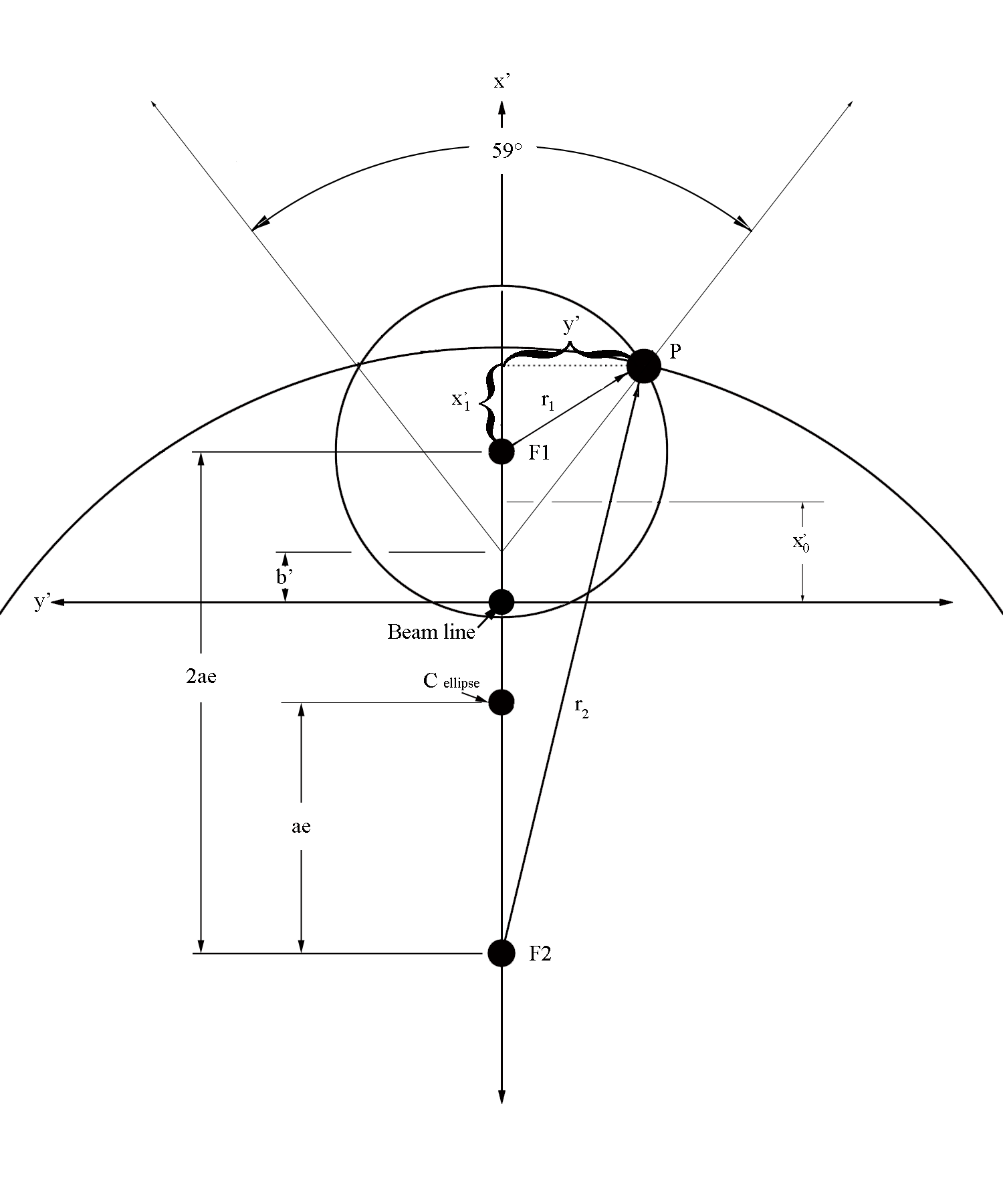
We can use the geometry of the sector to impose limits on the allowed x and y for this plane. The angle which the two sides of the triangle that make up the sector is given as [math]59^{\circ}[/math]. Each focii will have a ray that creates a circle around the point that is equal to the length found from the D1P and D2P lines. These circles will overlap at a common y component, which can be used to determine if the point is within the detector limits.
Using the physical constraints of the distance the interior walls of the side walls intersect each other from the beam line, as well as the angle the lowest guard wire at the plane midpoint.
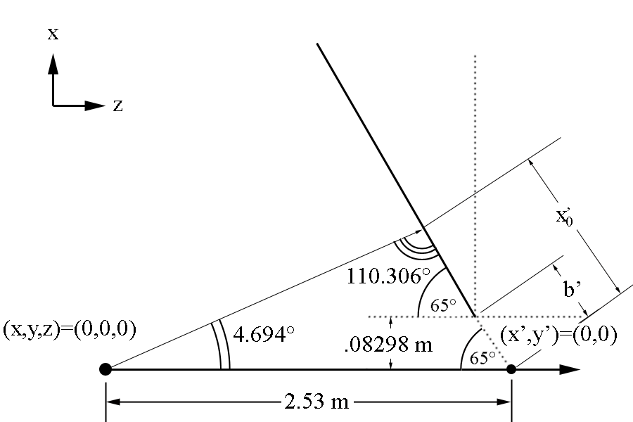
where b' is the location on the y' axis where the two interior side walls of the sector intersect.
[math]b'=\frac{0.08298\ m}{sin(65^{\circ})}=.09156\ m[/math]
The quantity [math]x_0^'[/math] is the corresponding x' distance from the beam line and detector plane intersection.
[math]\frac{x_0^'}{sin(4.694^{\circ})}=\frac{2.53\ m}{sin(110.306^{\circ})}[/math]
[math]x_0^'=\frac{sin(4.694^{\circ})2.53\ m}{sin(110.306^{\circ})}=.0872(2.53)=.22070/ m[/math]
Since the interior sides of the sector make an angle of [math]59^{\circ}[/math] in the plane of the wires, this can be represented by equations
[math]x'=\pm cot(29.5^{\circ})y^'+.09156\ m[/math]
Using the properties of an ellipse, we can work in the coordinates of the ellipse, in the plane of the ellipse, where the vertex is located at the crossing of the ellipse and the cone. Since the Dandelin construction was used, we know that
[math]F1P=D1P\qquad \text{and}\ F2P=D2P[/math]
If we shift the origin from the center of the ellipse to the intersection of the plane and cone for a given theta
[math]c_{ellipse}\equiv(-\Delta a,0)[/math]
[math]F1\equiv (-\Delta a+ae,0)\qquad F2\equiv (-\Delta a-ae,0)[/math]
Writing the equations for circles centered at an ellipse focii points, we find
[math]x_1^{'2}+y_1^{'2}=r_1^{'2}\qquad \qquad x_2+^{'2}+y_2^{'}2=r_2^{'2}[/math]
[math]r_1^{'2}-x_1^{'2}=y_1^{'2}\qquad \qquad y_2^{'2}=r_2^{'2}-x_2^{'2}[/math]
Since the focii are seperated by 2ae as found earlier
[math]x_2^'=x_1^'+2ae[/math]
[math]r_1^{'2}-x_1^{'2}=r_2^{'2}-(x_1^'+2ae)^2[/math]
[math]r_1^{'2}-r_2^{'2}=-4x_1^'ae-4a^2e^2[/math]
[math]r_2^{'2}-r_1^{'2}=8ae(x_1^'+ae+\Delta a)[/math]
[math]\frac{r_2^{'2}-r_1^{'2}}{4ae}-ae=x_1^'[/math]
Test for [math]\theta=20[/math] and [math]\phi=0[/math]
Substituting in the values found earlier for the case of [math]\theta=20^{\circ}[/math] and [math]\phi=0[/math]
[math]a=\frac{a_1+a_2}{2}=1.0459[/math]
[math]e\equiv \frac{sin(25^{\circ})}{cos(\theta)}= \frac{sin(25^{\circ})}{cos(20^{\circ})}=.4497[/math]
[math]x_1^'=\frac{r_2^{'2}-r_1^{'2}}{4ae}-ae=\frac{r_2^{'2}-r_1^{'2}}{4(1.0459)(.4497)}-(1.0459)(.4497)[/math]
Since
[math]\lVert \overrightarrow{D1P} \rVert \equiv \lVert \overrightarrow{F1P} \rVert \qquad \qquad \lVert \overrightarrow{D2P} \rVert \equiv \lVert \overrightarrow{F2P} \rVert[/math]
[math]D1P \approx .576\ \text{m}\qquad D2P \approx 1.516\ \text{m}[/math]
The [math]x_1^' [/math] distance from focal point 1 is:
[math]x_1^'=\frac{1.516^2-.576^2}{4(1.0459)(.4497)}-(1.0459)(.4497)=\frac{1.97}{1.88}-.4703=.576\ \text{m}=r_1[/math]
This is the radius from focal point 1, which is to be expected since the y component is equal to zero for [math]\phi=0[/math]
The focii are located at
[math]F1\equiv (-\Delta a+ae,0)=(-.1775+1.0459(.4497),0)=(.292,0)\ \text{m}\qquad F2\equiv (-\Delta a-ae,0)=(-.1775-1.0450(.4497),0)=(-6.478,0)\ \text{m}[/math]
This implies that with respect to the origin, x', we find
[math]x'=x_1'+\Delta a+ae=.576+.292=.868\ \text{m}[/math]
Test for [math]\theta=20[/math] and [math]\phi=1[/math]
All previous quantities where calculated for [math]\theta=20^{\circ}[/math] and do not depend on the angle [math]\phi[/math]. The quantities that do change
| [math]x_{D1}=r_{D1}\ cos(\phi)=.5901cos(1^{\circ}))=.5900\text {m}\qquad y_{D1}=r_{D1}cos(\phi)=.5901 sin(1^{\circ}))=.0103\qquad z_{D1}=r_{D1} cot(\theta)=.5901cot(20)=1.6212\ \text{m}[/math]
|
| [math]x_{D2}=r_{D2} cos(\phi)=1.3055cos(1^{\circ}))=1.3053\text {m}\qquad y_{D2}=r_{D2} sin(\phi)=1.3055sin(1^{\circ}))=.0228\qquad z_{D2}=r_{D2} cot(\theta)=1.3055cot(20)=3.5868\ \text{m}[/math]
|
| [math]x_P=\frac{2.53cos(\phi)}{(cot(\theta)+cos(\phi)cot(65^{\circ})}=\frac{2.53cos(1^{\circ}))}{(cot(20^{\circ})+cos(1^{\circ}))cot(65^{\circ})}=0.7869[/math]
|
| [math]y_P=\frac{2.53sin(\phi)}{(cot(\theta)+cos(\phi)cot(65^{\circ})}=\frac{2.53sin(1^{\circ}))}{(cot(20^{\circ})+cos(1^{\circ}))cot(65^{\circ})}=.0137[/math]
|
| [math]z_P=\frac{2.53cot(\theta)}{(cot(\theta)+cos(\phi)cot(65^{\circ})}=\frac{2.53cot(20^{\circ})}{(cot(20^{\circ})+cos(1^{\circ}))cot(65^{\circ})}=2.1624[/math]
|
[math]D2P=\sqrt{(x_{D2}-x_P)^2+(y_{D2}-y_P)^2+(z_{D2}-z_P)^2}=\sqrt{(1.3053-0.7869)^2+(.0228-.0137)^2+(3.5868-2.1624)^2}=\sqrt{(.5184)^2+(.0091)^2+(1.4244)^2}=1.51582872713\ \text{m}[/math]
[math]D1P=\sqrt{(x_P-x_{D1})^2+(y_P-y_{D1})^2+(z_P-z_{D1})^2}=\sqrt{(0.7871-.5900)^2+(.0137-.0103)^2+(2.1624-1.6212)^2}=\sqrt{(.1971)^2+(.0034)^2+(.5412)^2}=.575983862621\ \text{m}[/math]
[math]x_1^'=\frac{r_2^{'2}-r_1^{'2}}{4ae}-ae=\frac{1.5158^{'2}-.5758^{'2}}{4(1.0459)(.4497)}-(1.0459)(.4497)=.575\ \text{m}[/math]
Using the pythagorean theorem
[math]y'=\sqrt{.576^2-.575^2}=.03\ \text{m}[/math]
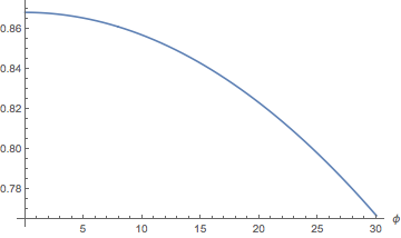
The two possible answers denote shifting to the left on right on the y axis. We take the direction of positive and negative to be the same as the sign convention for the angle phi starting on the x axis and shifting positive clockwise. A shift of 1 degree in phi at theta equal to 20 degrees only results in a small change in the x and y. This changes depending on the angles.
Function for the change in x' in the detector frame for change in [math]\phi[/math] and constant [math]\theta[/math] in the lab frame
[math]D2P=\sqrt{(x_{D2}-x_P)^2+(y_{D2}-y_P)^2+(z_{D2}-z_P)^2}[/math]
[math]D1P=\sqrt{(x_P-x_{D1})^2+(y_P-y_{D1})^2+(z_P-z_{D1})^2}[/math]
[math]x_1^'=\frac{((x_{D2}-x_P)^2+(y_{D2}-y_P)^2+(z_{D2}-z_P)^2)-((x_P-x_{D1})^2+(y_P-y_{D1})^2+(z_P-z_{D1})^2)}{4ae}-ae[/math]
| [math]x_{D1}=r_{D1}\ cos(\phi)\qquad y_{D1}=r_{D1}cos(\phi)\qquad z_{D1}=r_{D1} cot(\theta)[/math]
|
| [math]x_{D2}=r_{D2} cos(\phi)\qquad y_{D2}=r_{D2} sin(\phi)\qquad z_{D2}=r_{D2} cot(\theta)[/math]
|
| [math]x_P=\frac{2.53cos(\phi)}{(cot(\theta)+cos(\phi)cot(65^{\circ})}[/math]
|
| [math]y_P=\frac{2.53sin(\phi)}{(cot(\theta)+cos(\phi)cot(65^{\circ})}[/math]
|
| [math]z_P=\frac{2.53cot(\theta)}{(cot(\theta)+cos(\phi)cot(65^{\circ})}[/math]
|
[math]x_1^'=\frac{((x_{D2}-x_P)^2+(y_{D2}-y_P)^2+(z_{D2}-z_P)^2)-((x_P-x_{D1})^2+(y_P-y_{D1})^2+(z_P-z_{D1})^2)}{4ae}-ae[/math]
[math]x_1^'=\frac{x_{D2}^2-2x_Px_{D2}+x_P^2+y_{D2}^2-2y_Py_{D2}+y_P^2+z_{D2}^2-2z_Pz_{D2}+z_P^2-x_P^2+2x_Px_{D1}-x_{D1}^2-y_P^2+2y_Py_{D1}-y_{D1}^2-z_P^2+2z_Pz_{D1}-z_{D1}^2}{4ae}-ae[/math]
[math]x_1^'=\frac{(x_{D2}^2+y_{D2}^2)-(x_{D1}^2+y_{D1}^2)+z_{D2}^2-z_{D1}^2-2x_P(x_{D2}-x_{D1})-2y_P(y_{D2}-y_{D1})-2z_P(z_{D2}-z_{D1})}{4ae}-ae[/math]
[math]x_1^'=\frac{(r_{D2}^2)-(r_{D1}^2)+cot^2(\theta)(r_{D2}^2-r_{D1}^2)-2x_P(x_{D2}-x_{D1})-2y_P(y_{D2}-y_{D1})-2z_P(z_{D2}-z_{D1})}{4ae}-ae[/math]
Expressing this as functions of [math]\phi[/math] and non-differentiable constants
[math]x_1^'=\frac{c_1+c_2-2x_P(\phi)x_{D2}(\phi)+2x_P(\phi)x_{D1}(\phi)-2y_P(\phi)y_{D2}(\phi)+2y_P(\phi)y_{D1}(\phi)-2z_P(\phi)c_3}{4c_4}-c_4[/math]
Differentiating with respect to [math]\phi[/math]
| [math]x_{D1}=r_{D1} cos(\phi)\Rightarrow \dot x_{D1}=-r_{D1} sin(\phi)[/math]
|
| [math]y_{D1}=r_{D1}sin(\phi)\Rightarrow \dot y_{D1}=r_{D1}cos(\phi)[/math]
|
| [math]x_{D2}=r_{D2} cos(\phi)\Rightarrow \dot x_{D2}=-r_{D2} sin(\phi)[/math]
|
| [math]y_{D2}=r_{D2}sin(\phi)\Rightarrow \dot y_{D2}=r_{D2}cos(\phi)[/math]
|
| [math]x_P=\frac{2.52934271645cos(\phi)}{cot(\theta)+cos(\phi)cot(65^{\circ})}\Rightarrow \dot x_P=\frac{-2.52934271645cot(\theta)sin(\phi)}{(cos(\phi)cot(65^{\circ}+cot(\theta))^2}[/math]
|
| [math]y_P=\frac{2.52934271645sin(\phi)}{cot(\theta)+cos(\phi)cot(65^{\circ})}\Rightarrow \dot y_P=\frac{-1.7206+2.52934271645 cos(\phi) cot(\theta)}{(cos(\phi) cot(65^{\circ}) + cot(\theta))^2}[/math]
|
| [math]z_P=\frac{2.52934271645cot(\theta)}{cot(\theta)+cos(\phi)cot(65^{\circ})}\Rightarrow \dot z_P=\frac{-1.7206 cot(\theta)sin(\phi))}{(cos(\phi) cot(65) + cot(\theta))^2}[/math]
|
[math]\frac{dx_1^1}{d\phi}=\frac{-2}{4c_4}\frac{d}{d\phi}(x_P(\phi)x_{D2}(\phi))+\frac{2}{4c_4}\frac{d}{d\phi}(x_P(\phi)x_{D1}(\phi))-\frac{2}{4c_4}\frac{d}{d\phi}(y_P(\phi)y_{D2}(\phi))+\frac{2}{4c_4}\frac{d}{d\phi}(y_P(\phi)y_{D1}(\phi))-\frac{2c_3}{4c_4}\frac{d}{d\phi}z_P(\phi)[/math]
[math]\frac{dx_1^1}{d\phi}=\frac{-2}{4c_4} \left ( (\dot x_P(\phi)x_{D2}(\phi)+x_P(\phi)\dot x_{D2}(\phi))-(\dot x_P(\phi)x_{D1}(\phi)+x_P(\phi)\dot x_{D1}(\phi))+(\dot y_P(\phi)y_{D2}(\phi)+y_P(\phi)\dot y_{D2}(\phi))-(\dot y_P(\phi)y_{D1}(\phi)+y_P(\phi)\dot y_{D1}(\phi))+c_3\dot z_P(\phi) \right )[/math]
Function for the wire number in the detector frame for change in [math]\phi[/math] and constant [math]\theta[/math] in the lab frame
Using the expression for wire number n in terms of [math]\theta[/math] for the detector mid-plane where [math]\phi=0[/math]:
[math]n = \frac{-957.412}{\tan(\theta)+2.14437}+430.626[/math]
We can use the inverse of this function to find the neighboring wire's corresponding angle theta
[math]\theta\equiv 4.49876 +0.293001 n+0.000679074 n^2-3.57132\times 10^{-6} n^3[/math]
[math]\theta(n \pm 1)\equiv 4.49876 +0.293001 (n \pm 1)+0.000679074 (n \pm 1)^2-3.57132\times 10^{-6} (n \pm 1)^3[/math]
We also know what the x' function must follow dependent on phi in the detector plane
[math]x_1^'=\frac{((x_{D2}-x_P)^2+(y_{D2}-y_P)^2+(z_{D2}-z_P)^2)-((x_P-x_{D1})^2+(y_P-y_{D1})^2+(z_P-z_{D1})^2)}{4ae}-ae[/math]
[math]x_1^'=\frac{(r_{D2}^2)-(r_{D1}^2)+cot^2(\theta)(r_{D2}^2-r_{D1}^2)-2x_P(x_{D2}-x_{D1})-2y_P(y_{D2}-y_{D1})-2z_P(z_{D2}-z_{D1})}{4ae}-ae[/math]
| [math]x_{D1}=r_{D1}\ cos(\phi)\qquad y_{D1}=r_{D1}cos(\phi)\qquad z_{D1}=r_{D1} cot(\theta)[/math]
|
| [math]x_{D2}=r_{D2} cos(\phi)\qquad y_{D2}=r_{D2} sin(\phi)\qquad z_{D2}=r_{D2} cot(\theta)[/math]
|
| [math]x_P=\frac{2.53cos(\phi)}{(cot(\theta)+cos(\phi)cot(65^{\circ})}[/math]
|
| [math]y_P=\frac{2.53sin(\phi)}{(cot(\theta)+cos(\phi)cot(65^{\circ})}[/math]
|
| [math]z_P=\frac{2.53cot(\theta)}{(cot(\theta)+cos(\phi)cot(65^{\circ})}[/math]
|
[math]r_{D1}=R_{Lower\ Dandelin}cos(\theta)=(ae-\Delta a) tan(65^{\circ})cos(\theta)\qquad \qquad r_{D2}=R_{Lower\ Dandelin}cos(\theta)=(ae+\Delta a) tan(65^{\circ})cos(\theta)[/math]
We can take this point to be the x axis intercept and use the fact that each wire is titled by 6 degrees to the horizontal in the plane of the detector to create an equation
[math]x_{wire\ n}'=tan(6^{\circ})y'+x_{n_0}[/math]
where the initial wire and x' position at the given theta is represented by [math]n_0[/math]
[math]x_{n0}=x'+\Delta x'\ n[/math]
[math]x'=\frac{x}{z}\qquad \Delta x'=\frac{\Delta x}{\Delta z}[/math]
\[Theta]=20;
\[CapitalDelta]a=(2.52934271645Sin[\[Theta] \[Degree]])/2 (Csc[65\[Degree]-\[Theta] \[Degree]]-Csc[115\[Degree]-\[Theta] \[Degree]]);

e=Sin[25\[Degree]]/Cos[\[Theta] \[Degree]];

a=(2.52934271645Sin[\[Theta] \[Degree]])/2 (Csc[65 \[Degree]-\[Theta] \[Degree]]+Csc[115 \[Degree]-\[Theta] \[Degree]]);

rD1=(a e-\[CapitalDelta]a) Tan[65\[Degree]]Cos[\[Theta] \[Degree]];

rD2=(a e+\[CapitalDelta]a) Tan[65\[Degree]]Cos[\[Theta] \[Degree]];


xD1=rD1 Cos[\[Phi] \[Degree]];

yD1=rD1 Sin[\[Phi] \[Degree]];

zD1=rD1 Cot[\[Theta] \[Degree]];

xD2=rD2 Cos[\[Phi] \[Degree]];

 yD2=rD2 Sin[\[Phi] \[Degree]];

 zD2=rD2 Cot[\[Theta] \[Degree]];

xP=(2.52934271645Cos[\[Phi] \[Degree]])/(Cot[\[Theta] \[Degree]]+Cos[\[Phi] \[Degree]]Cot[65\[Degree]]);

yP=(2.52934271645Sin[\[Phi] \[Degree]])/(Cot[\[Theta] \[Degree]]+Cos[\[Phi] \[Degree]]Cot[65\[Degree]]);

zP=(2.52934271645Cot[\[Theta] \[Degree]])/(Cot[\[Theta] \[Degree]]+Cos[\[Phi] \[Degree]]Cot[65\[Degree]]);

x1=(rD2^2-rD1^2+Cot[\[Theta] \[Degree]]^2 (rD2^2-rD1^2)-2xP(xD2-xD1)-2yP(yD2-yD1)-2zP(zD2-zD1))/(4a e)-a e;
x=x1-\[CapitalDelta]a+a e//N;
n= -957.412/(Tan[\[Theta] \[Degree]]+2.14437)+430.626
D1P=Sqrt[(xP-xD1)^2+(yP-yD1)^2+(zP-zD1)^2];
y=Sqrt[D1P^2-x^2]//N;
As discussed earlier, taking the 1st derivative of this function will give us the spacing of the bins as a function of wire number.
[math]\theta '\equiv 0.293001 + 0.00135815 n - 0.000010714 n^2[/math]