|
|
| Line 7: |
Line 7: |
| | ==Simulation Setup== | | ==Simulation Setup== |
| | Determine the Moller background using an [[LH2 target]] to check the physics in GEANT4 | | Determine the Moller background using an [[LH2 target]] to check the physics in GEANT4 |
| − |
| |
| − | ===Working with Moller Data===
| |
| − | The event data from the GEANT4 simulation is written to a data file in the following format:
| |
| − |
| |
| − | {| border="1" align=center
| |
| − | |-
| |
| − | ! KE<sub>i</sub>
| |
| − | ! Px<sub>i</sub>
| |
| − | ! Py<sub>i</sub>
| |
| − | ! Pz<sub>i</sub>
| |
| − | ! x<sub>i</sub>
| |
| − | ! y<sub>i</sub>
| |
| − | ! z<sub>1</sub>
| |
| − | ! KE<sub>f</sub>
| |
| − | ! Px<sub>f</sub>
| |
| − | ! Py<sub>f</sub>
| |
| − | ! Pz<sub>f</sub>
| |
| − | ! x<sub>f</sub>
| |
| − | ! y<sub>f</sub>
| |
| − | ! z<sub>f</sub>
| |
| − | ! KE<sub>m</sub>
| |
| − | ! Px<sub>m</sub>
| |
| − | ! Py<sub>m</sub>
| |
| − | ! Pz<sub>m</sub>
| |
| − | ! x<sub>m</sub>
| |
| − | ! y<sub>m</sub>
| |
| − | ! z<sub>m</sub>
| |
| − | |-
| |
| − | | 11000
| |
| − | | 0
| |
| − | | 0
| |
| − | | 11000.5
| |
| − | | 0
| |
| − | | 0
| |
| − | | -510
| |
| − | | 10999.1
| |
| − | | 0.433025
| |
| − | | -0.858867
| |
| − | | 10999.6
| |
| − | | 0
| |
| − | | 0
| |
| − | | -509.276
| |
| − | | 0.905324
| |
| − | | -0.433025
| |
| − | | 0.858867
| |
| − | | 0.905366
| |
| − | | 0
| |
| − | | 0
| |
| − | | -509.276
| |
| − | |}
| |
| − | <center>'''Table 1:'''Data format for Moller events in GEANT4 simulation. "i" represents the incoming electron, "f" represents the scattered, or final state, of the incoming electron, and "m" stands for the Moller electron.</center>
| |
| − |
| |
| − |
| |
| − | Where each line represents a Moller scattering with the kinematic variables of kinetic energy, momentum in the x, y, and z directions, as well as the x, y, and z position of the collision for the Incoming electron, the scattered state of the incoming electron, and the scattered Moller electron in that specific order.
| |
| − |
| |
| − |
| |
| − | Using a c++ macro, the variables are read into a Root tree, with branches for each variable. Specific histograms are also created for the total momentum and the scattering angle theta for the scattered and Moller electron, both in the Lab frame and Center of Mass frame.
| |
| − |
| |
| − | <pre>
| |
| − | tree->Branch("evt",&evt.event,"event/I:IntKE/F:IntPx:IntPy:IntPz:IntPosx:IntPosy:IntPosz:FnlKE:FnlPx:FnlPy:FnlPz:FnlPosx:FnlPosy:FnlPosz:
| |
| − | MolKE:MolPx:MolPy:MolPz:MolPosx:MolPosy:MolPosz");
| |
| − | while(in.good())
| |
| − | {
| |
| − | //Create Tree from GEANT4 simulation data
| |
| − | evt.event=nlines;
| |
| − | in >> evt.IntKE >> evt.IntMom[0] >> evt.IntMom[1] >> evt.IntMom[2] >> evt.IntPos[0]
| |
| − | >> evt.IntPos[1] >> evt.IntPos[2] >> evt.FnlKE >> evt.FnlMom[0] >> evt.FnlMom[1] >> evt.FnlMom[2]
| |
| − | >> evt.FnlPos[0] >> evt.FnlPos[1] >> evt.FnlPos[2] >> evt.MolKE >> evt.MolMom[0] >> evt.MolMom[1]
| |
| − | >> evt.MolMom[2] >> evt.MolPos[0] >> evt.MolPos[1] >> evt.MolPos[2];
| |
| − |
| |
| − | nlines++;
| |
| − |
| |
| − | tree->Fill();
| |
| − |
| |
| − | FnlE=sqrt(evt.FnlMom[0]*evt.FnlMom[0]+evt.FnlMom[1]*evt.FnlMom[1]+evt.FnlMom[2]*evt.FnlMom[2]+0.511*0.511);
| |
| − | IntE=sqrt(evt.IntMom[0]*evt.IntMom[0]+evt.IntMom[1]*evt.IntMom[1]+evt.IntMom[2]*evt.IntMom[2]+0.511*0.511);
| |
| − | MolE=sqrt(evt.MolMom[0]*evt.MolMom[0]+evt.MolMom[1]*evt.MolMom[1]+evt.MolMom[2]*evt.MolMom[2]+0.511*0.511);//Define 4Vectors
| |
| − | Fnl4Mom.SetPxPyPzE(evt.FnlMom[0],evt.FnlMom[1],evt.FnlMom[2],FnlE);
| |
| − | Int4Mom.SetPxPyPzE(evt.IntMom[0],evt.IntMom[1],evt.IntMom[2],IntE);
| |
| − | Mol4Mom.SetPxPyPzE(evt.MolMom[0],evt.MolMom[1],evt.MolMom[2],MolE);
| |
| − |
| |
| − | //Create Lab Frame Histograms
| |
| − | FinalMomentum->Fill(Fnl4Mom.P());
| |
| − | MollerMomentum->Fill(Mol4Mom.P());
| |
| − | FinalTheta->Fill(Fnl4Mom.Theta()*180/3.14);
| |
| − | MollerTheta->Fill(Mol4Mom.Theta()*180/3.14);
| |
| − | //Boost to Center of Mass Frame
| |
| − | CMS=Fnl4Mom+Mol4Mom;
| |
| − | Fnl4Mom.Boost(-CMS.BoostVector());
| |
| − |
| |
| − | Mol4Mom.Boost(-CMS.BoostVector());
| |
| − | //Create CM Histograms
| |
| − | FinalMomentumCM->Fill(Fnl4Mom.P());
| |
| − | MollerMomentumCM->Fill(Mol4Mom.P());
| |
| − | FinalThetaCM->Fill(Fnl4Mom.Theta()*180/3.14);
| |
| − | MollerThetaCM->Fill(Mol4Mom.Theta()*180/3.14);
| |
| − | }
| |
| − | </pre>
| |
| | | | |
| | =='Momentum distributions in the Lab Frame == | | =='Momentum distributions in the Lab Frame == |
need to insert moller shielding into card after moller LUND file is created. (see clas12/beamline)
Simulating the Moller scattering background for EG12
GEANT4 Simulation of Moller Events
Simulation Setup
Determine the Moller background using an LH2 target to check the physics in GEANT4
'Momentum distributions in the Lab Frame
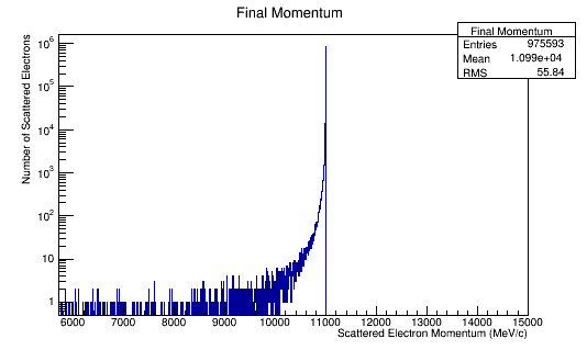
Figure 1a: The scattered electron momentum distribution for 4E7 incident 11 GeV electrons in the Lab frame of reference.
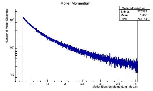
Figure 1b: The Moller electron momentum distribution for 4E7 incident 11 GeV electrons in the Lab frame of reference.
Angular Distribution in the Lab Frame
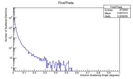
Figure 2a: The scattered electron scattering angle theta distribution for 4E7 incident 11 GeV electrons in the Lab frame of reference.
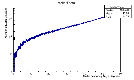
Figure 2b: The Moller electron scattering angle theta distribution for 4E7 incident 11 GeV electrons in the Lab frame of reference.
Momentum distributions in the Center of Mass Frame
Estimated Momentum Distribution
Noting that the GEANT4 data included data for the Kinetic Energy and not the total energy, we can perform the substitution using
[math]E^2=p^2+m^2[/math]
Performing the relativistic transformation, we find for an incoming electron with momentum of 11GeV, we should find the momentum in the center of mass to be around 53 MeV .
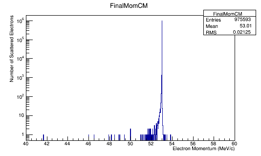
Figure 3a: The scattered electron momentum distribution for 4E7 incident 11 GeV(Lab) electrons in the Center of Mass frame of reference.
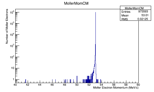
Figure 3b: The Moller electron momentum distribution for 4E7 incident 11 GeV(Lab) electrons in the Center of Mass frame of reference.
Angular Distribution in the Center of Mass Frame
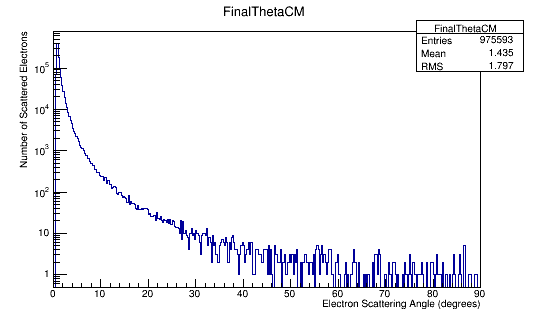
Figure 4a: The scattered electron scattering angle theta distribution for 4E7 incident 11 GeV(Lab) electrons in the Center of Mass frame of reference.
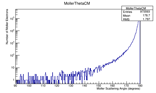
Figure 4b: The Moller electron scattering angle theta distribution for 4E7 incident 11 GeV(Lab) electrons in the Center of Mass frame of reference.
Comparing experimental vs. theoretical for Møller differential cross section 11GeV
Using the equation from [1]
[math]\frac{d\sigma}{d\Omega}=\frac{ e^4 }{8E^2}\left \{\frac{1+cos^4\frac{\theta}{2}}{sin^4\frac{\theta}{2}}+\frac{1+sin^4\frac{\theta}{2}}{cos^4\frac{\theta}{2}}+\frac{2}{sin^2\frac{\theta}{2}cos^2\frac{\theta}{2}} \right \}[/math]
where [math]\alpha=\frac{e^2}{\hbar c}\quad with\quad \hbar = c =1[/math]
This can be simplified to the form
[math]\frac{d\sigma}{d\Omega}=\frac{ \alpha^2 }{4E^2}\frac{ (3+cos^2\theta)^2}{sin^4\theta}[/math]
Plugging in the values expected for a scattering electron:
[math]\alpha ^2=5.3279\times 10^{-5}[/math]
[math]E\approx 53 MeV[/math]
Using unit analysis on the term outside the parantheses, we find that the differential cross section for an electron at this momentum should be around
[math]\frac{5.3279\times 10^{-5}}{4\times 2.81\times 10^{15}eV^2}=4.74\times 10^{-21} eV^{-2}=\frac{4.74\times 10^{-21}}{1eV^2}\times \frac{1\times 10^{18}eV^2 }{1\ GeV^2}=\frac{.0047}{GeV^2}[/math]
Using the conversion of
[math]\frac{1}{1GeV^2}=.3894 mb[/math]
[math]\frac{1\ GeV^{-2}}{.3894\ mb}=\frac{.0047\ GeV^{-2}}{x\ mb}[/math]
The trigonometric function part of the equation comes out to it's minimum of 9 at 90 degrees.
[math]\frac{(3+Cos^2(90))^2}{Sin^4(90)}=9[/math]
We find that the differential cross section scale is [math]\frac{d\sigma}{d\Omega}\approx 1.8\times 10^{-3}mb \times 9=16.2\mu b[/math]
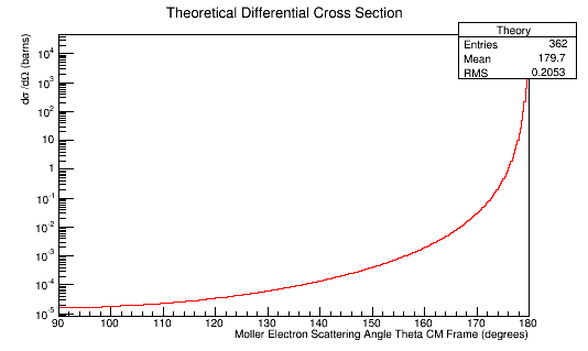
Figure 5a: The theoretical Moller electron differential cross-section for an incident 11 GeV(Lab) electron in the Center of Mass frame of reference.
Converting the number of electrons scattered per angle theta to barns, we can use the relation
[math]L=\frac{i_{scattered}}{\sigma} \approx i_{scattered}\times \rho_{target}\times l_{target}[/math]
where ρtarget is the density of the target material, ltarget is the length of the target, and iscattered is the number of incident particles scattered.
This gives, for LH2:
[math]\rho_{target}\times l_{target}=\frac{70.85 kg}{1 m^3}\times \frac{1 mole}{2.02 g} \times \frac{1000g}{1 kg} \times \frac{6\times10^{23} atoms}{1 mole} \times \frac{1m^3}{(100 cm)^3} \times \frac{1 cm}{ } \times \frac{10^{-24} cm^{2}}{barn} =2.10\times 10^{-2} barns[/math]
Using the number of incident electrons,
[math]\frac{1}{\rho_{target}\times l_{target} \times 4\times 10^7}=1.19\times 10^{-6} barns[/math]
We can use this number to scale the number of electrons per angle to a differential cross-section in barns. Using the plot of the Moller electron scattering angle theta in the Center of Mass frame,
Figure 5b: The Moller electron scattering angle theta distribution for an incident 11 GeV(Lab) electron in the Center of Mass frame of reference.
We can rescale and combine the theoretical differential cross-section for one electron.
TH1F *Combo=new TH1F("TheoryExperiment","Theoretical and Experimental Differential Cross-Section CM Frame",360,90,180);
Combo->Add(MollerThetaCM,1.19e-6);
Combo->Draw();
Theory->Draw("same");
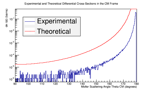
Figure 5c: The experimental and theoretical Moller electron differential cross-section for an incident 11 GeV(Lab) electron in the Center of Mass frame of reference.
Change to a NH3 Target
Replacing the LH2 target with an NH3 target in the ExN02DectectorConstruction.cc file
//Ammonia
G4Element* N = new G4Element("Nitrogen", "N", z=7., a=14.01*g/mole);
G4Element* H = new G4Element("Hydrogen","H",z=1.,a=1.01*g/mole);
G4Material* NH3 = new G4Material("Ammonia", density=0.86*g/cm3, ncomponents=2,kStateGas, temperature, pressure);
NH3->AddElement(N,natoms=1);
NH3->AddElement(H,natoms=3);
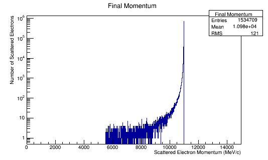
Figure 6a: The scattered electron momentum distribution for 4E7 incident 11 GeV electrons in the Lab frame of reference.
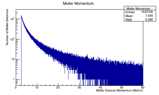
Figure 6b: The Moller electron momentum distribution for 4E7 incident 11 GeV electrons in the Lab frame of reference.
Increasing the number of incident electrons, Moller Momentum now appears as:
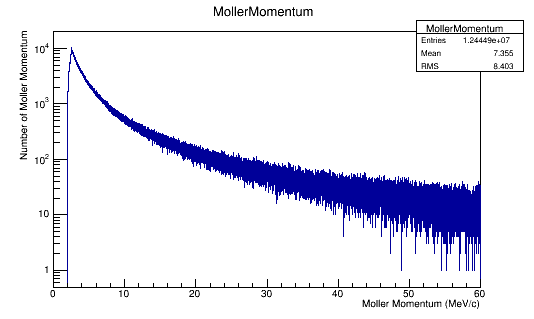
Figure 6c: The Moller electron momentum distribution for 4E8 incident 11 GeV electrons in the Lab frame of reference.

Figure 6d: The scattered electron momentum distribution for 4E7 incident 11 GeV(Lab) electrons in the Center of Mass frame of reference.
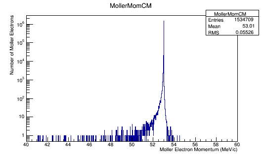
Figure 6e: The Moller electron momentum distribution for 4E7 incident 11 GeV(Lab) electrons in the Center of mass frame of reference.
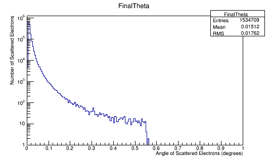
Figure 6f: The Moller electron scattering angle thetea distribution for 4E7 incident 11 GeV electrons in the Lab frame of reference.

Figure 6g: The Moller electron scattering angle theta distribution for 4E7 incident 11 GeV electrons in the Lab frame of reference.
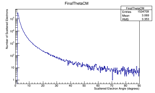
Figure 6h: The Scattered electron scattering angle theta distribution for 4E7 incident 11 GeV(Lab) electrons in the Center of Mass frame of reference.
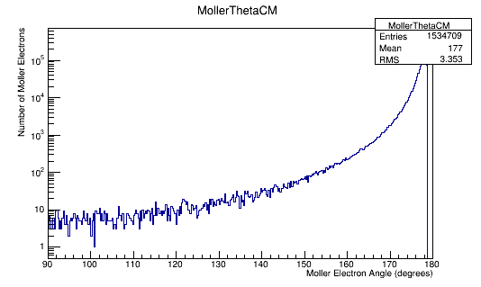
Figure 6i: The Moller electron scattering angle theta distribution for 4E7 incident 11 GeV(Lab) electrons in the Center of Mass frame of reference.
LH2 Vs. NH3
Plotting the Momentum and Scattering angle Theta in the Lab and Center of Mass frame of reference for LH2 and NH3 targets.
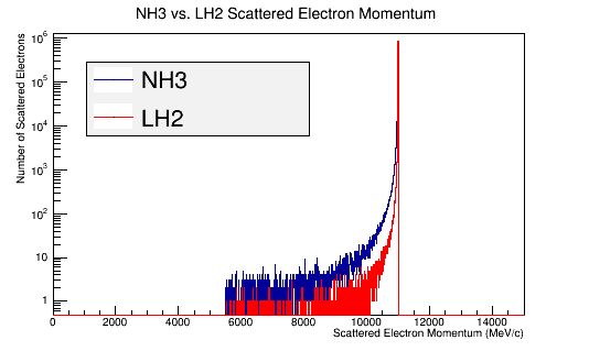
Figure 7a: The scattered electron momentum distribution for 4E7 incident 11 GeV electrons in the Lab frame of reference.
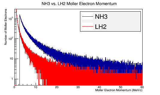
Figure 7b: The Moller electron momentum distribution for 4E7 incident 11 GeV electrons in the Lab frame of reference.
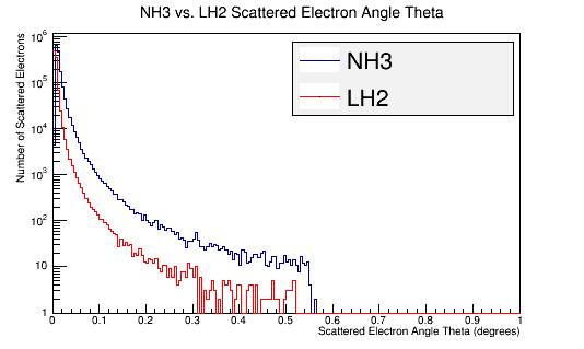
Figure 7c: The Scattered electron scattering angle theta distribution for 4E7 incident 11 GeV electrons in the Lab frame of reference.
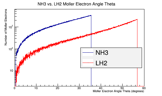
Figure 7d: The Moller electron scattering angle theta distribution for 4E7 incident 11 GeV electrons in the Lab frame of reference.
Figure out the offset
Rerunning the GEANT simulation for a target of solo atoms of Carbon 12
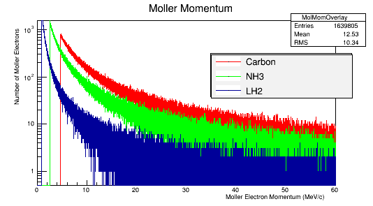
Figure 8a: The scattered electron momentum distribution for 4E7 incident 11 GeV electrons in the Lab frame of reference.
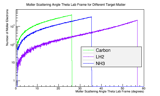
Figure 8b: The Moller electron momentum distribution for 4E7 incident 11 GeV electrons in the Lab frame of reference.
These graphs show an offset based upon the density of the target material.
Density of target material
C=2.26 g/cm3
NH3=.86g/cm3
LH2=.07g/cm3
[math]\Longrightarrow[/math]The greater the density, the smaller the solid angle into which the Moller electron will scatter.
Density, atomic mass, and electron number effects
Temporarily changing the density of LH2 to be .86g/cm3, the density of NH3, and altering the atomic mass and electron number, we find
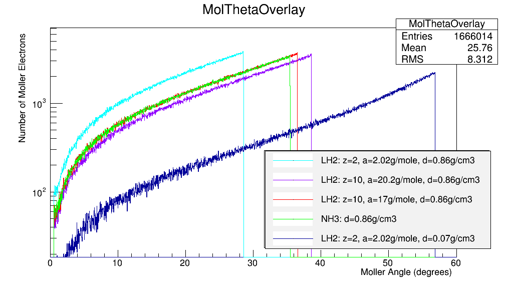
Figure 8c: The Moller electron scattering angle theta distribution for 4E7 incident 11 GeV electrons in the Lab frame of reference.
Differential Cross-Section Offset
Comparing this to the theoretical differential cross section:
As shown above , we find that the differential cross section scale is [math]\frac{d\sigma}{d\Omega}\approx 16.2\times 10^{-2}mb=16.2\mu b[/math]
Converting the number of electrons to barns,
[math]L=\frac{i_{scattered}}{\sigma} \approx i_{scattered}\times \rho_{target}\times l_{target}[/math]
where ρtarget is the density of the target material, ltarget is the length of the target, and iscattered is the number of incident particles scattered.
For LH2:
[math]\rho_{target}\times l_{target}=\frac{70.85 kg}{1 m^3}\times \frac{1 mole}{2.02 g} \times \frac{1000g}{1 kg} \times \frac{6\times10^{23} atoms}{1 mole} \times \frac{1m^3}{(100 cm)^3} \times \frac{1 cm}{ } \times \frac{10^{-24} cm^{2}}{barn} =2.10\times 10^{-2} barns[/math]
[math]\frac{1}{\rho_{target}\times l_{target} \times 4\times 10^7}=1.19\times 10^{-6} barns[/math]
For Carbon:
[math]\rho_{target}\times l_{target}=\frac{2.26 g}{1 cm^3}\times \frac{1 mole}{12.0107 g} \times \times \frac{6\times10^{23} atoms}{1 mole} \times \frac{1 cm}{ } \times \frac{10^{-24} cm^{2}}{barn} =1.13\times 10^{-1} barns[/math]
[math]\frac{1}{\rho_{target}\times l_{target} \times 4\times 10^7}=2.21\times 10^{-7} barns[/math]
For Ammonia:
[math]\rho_{target}\times l_{target}=\frac{.8 g}{1 cm^3}\times \frac{1 mole}{17 g} \times \frac{6\times10^{23} atoms}{1 mole} \times \frac{1 cm}{ } \times \frac{10^{-24} cm^2}{barn} =2.82\times 10^{-2} barns[/math]
[math]\frac{1}{\rho_{target}\times l_{target} \times 4\times 10^7}=8.87\times 10^{-7} barns[/math]
Combing plots in Root:
new TBrowser();
TH1F *LH2=new TH1F("LH2","LH2",360,90,180);
LH2->Add(MollerThetaCM,1.19e-6);
LH2->Draw();

TH1F *C12=new TH1F("C12","C12",360,90,180);
C12->Add(MollerThetaCM,2.21e-7);
C12->Draw();

TH1F *NH3=new TH1F("NH3","NH3",360,90,180);
NH3->Add(MollerThetaCM,8.87e-7);
NH3->Draw();
LH2->Draw("same");
C12->Draw("same");
Theory->Draw("same");

Figure 8c: The Moller electron differential cross-section for 4E7 incident 11 GeV electrons in the Center of Mass frame of reference.
Reconstruction
Moller Track Reconstruction in eg12
Papers used
[1]Farrukh Azfar's Derivation of Moller Scattering
- File:FarrukAzfarMollerScatter.pdf
A polarized target for the CLAS detector
- File:PHY02-33.pdf
An investigation of the spin structure of the proton in deep inelastic scattering of polarized muons on polarized protons
- File:1819.pdf
QED Radiative Corrections to Low-Energy Moller and Bhabha Scattering
http://arxiv.org/abs/1602.07609
EG12


