DV RunGroupC Moller

need to insert moller shielding into card after moller LUND file is created. (see clas12/beamline)

Simulating the Moller scattering background for EG12

GEANT4 Simulation of Moller Events

Simulation Setup

Determine the Moller background using an LH2 target to check the physics in GEANT4

Detector Material and Construction

Using GEANT4, the ExampleN02 file was edited to run for a NH3 target. The file ExN02DetectorConstruction.cc was edited with

//--------- Material definition ---------
  
  G4double a, z;
  G4double density, temperature, pressure;

//Liquid Hydrogen
G4Material* LH2 = new G4Material("Hydrogen", z=2., a=2.02*g/mole,  density=0.07*g/cm3, kStateGas,3*kelvin,1.7e5*pascal);

The target is a cylinder with a 1.5 cm diameter and 1 cm thickness following dimensions listed on page 8 of File:PHY02-33.pdf

//--------- Sizes of the principal geometrical components (solids)  ---------

  NbOfChambers = 1;
  ChamberWidth = 1.5*cm;
  ChamberSpacing = 40*cm;
  
  fTrackerLength = (NbOfChambers+1)*ChamberSpacing; // Full length of Tracker
  fTargetLength  = 1.0 * cm;                        // Full length of Target

  TargetMater = NH3;
  ChamberMater = BadVacuum;
  
  
  //fWorldLength= 1.2 *(fTargetLength+fTrackerLength);
  fWorldLength= 1.2 *(10+fTrackerLength)+100 *cm;
  
  G4double targetSize  = 0.5*fTargetLength;    // Half length of the Target
  G4double trackerSize = 0.5*fTrackerLength;   // Half length of the Tracker

Recording Moller Events

Moller scattering does not have a GEANT4 specific setting, so the file ExN02SteppingVerbose.cc was edited to record only events that would correspond to Moller events. Since Moller scattering is simply electron-electron scattering, we can look for events where electron ionization is the process in the data stream. We will limit this to only particles with a parentID of 0 and 1 representing the parent and daughter (Moller) electrons. This eliminates second generation Moller scatterings, which only ocur about 2 times out of 1E6 incoming electrons. This method also eliminates Delta Rays or Knock-on-Electrons.

The file ExN02SteppingVerbose.cc is read for each step in the GEANT4 simulation, so recording the momentum, position, and energies of the electrons before and after the collision can be found in multiple loops.

On the first pass of SteppingVerbose, the data is recorded into a temporary variable set. The physical process of ionization occurs after the collision of the two electrons. This implies that the data could possible be the initial state of the incoming electron. This is read every time to be prepared for the subsequent pass where the process of ionization (scattering) is active.

void ExN02SteppingVerbose::StepInfo()
{
.
.
.
if(fTrack->GetDefinition()->GetPDGEncoding()==11 && fStep->GetPostStepPoint()->GetProcessDefinedStep()->GetProcessName()!="eIoni" && fTrack->GetParentID()==0)
    {
        Temp_Energy=fTrack->GetKineticEnergy();
        Temp_Mom_x=fTrack->GetMomentum().x();
        Temp_Mom_y=fTrack->GetMomentum().y();
        Temp_Mom_z=fTrack->GetMomentum().z();
        Temp_Pos_x=fTrack->GetPosition().x();
        Temp_Pos_y=fTrack->GetPosition().y();
        Temp_Pos_z=fTrack->GetPosition().z();
    }

On a pass afterwards, the data is read into a variable for the final state when the physical state is ionization, representing the Moller scattering. The the temporary variable is read into the initial state.

if( fTrack->GetDefinition()->GetPDGEncoding()==11 && fStep->GetPostStepPoint()->GetProcessDefinedStep()->GetProcessName()=="eIoni" && fTrack->GetParentID()==0)
    {
        Final_Energy= fTrack->GetKineticEnergy();
        Final_Mom_x=fTrack->GetMomentum().x();
        Final_Mom_y=fTrack->GetMomentum().y();
        Final_Mom_z=fTrack->GetMomentum().z();
        Final_Pos_x=fTrack->GetPosition().x();
        Final_Pos_y=fTrack->GetPosition().y();
        Final_Pos_z=fTrack->GetPosition().z();
       
        Init_Energy=Temp_Energy;
        Init_Mom_x=Temp_Mom_x; 
        Init_Mom_y=Temp_Mom_y; 
        Init_Mom_z=Temp_Mom_z; 
        Init_Pos_x=Temp_Pos_x; 
        Init_Pos_y=Temp_Pos_y; 
        Init_Pos_z=Temp_Pos_z;
        
        }

This will write the data to an external file only for a 1st generation daughter particle and an active trigger. Afterwards, the trigger is turned off so that the recording process can start again.

 
if(fTrack->GetDefinition()->GetPDGEncoding()==11 && fTrack->GetParentID()==1 && trigger==1 )
   {
     outfile
     //G4cout
       << Init_Energy<< "    "
       <<  Init_Mom_x << "     "
       <<  Init_Mom_y << "     "
       <<  Init_Mom_z << "     "
       <<  Init_Pos_x << "     "
       <<  Init_Pos_y << "     "
       <<  Init_Pos_z << "     "
       << Final_Energy << "     "
       <<  Final_Mom_x << "     "
       <<  Final_Mom_y << "     "
       <<  Final_Mom_z << "     "
       <<  Final_Pos_x << "     "
       <<  Final_Pos_y << "     "  
       <<  Final_Pos_z << "     "
       << Mol_Energy << "     "
       <<  Mol_Mom_x << "     "
       <<  Mol_Mom_y << "     "
       <<  Mol_Mom_z << "     "
       <<  Mol_Pos_x << "     "
       <<  Mol_Pos_y << "     "
       <<  Mol_Pos_z << "     "
       << G4endl;
  trigger=0;
   }
.
.
.
}

On a later pass, the condition that the parentID no longer represents the parent. This implies that the particle a Moller electron and the data is recorded into the Moller final state. The trigger is activated, which on the next pass of the program will allow a printout of all Moller Scattering data.

void ExN02SteppingVerbose::TrackingStarted()
{
.
.
.
if(fTrack->GetDefinition()->GetPDGEncoding()==11 && fTrack->GetParentID()>0)
   {
     Mol_Energy=fTrack->GetKineticEnergy();
     Mol_Mom_x=fTrack->GetMomentum().x();
     Mol_Mom_y=fTrack->GetMomentum().y();
     Mol_Mom_z=fTrack->GetMomentum().z();
     Mol_Pos_x=fTrack->GetPosition().x();
     Mol_Pos_y=fTrack->GetPosition().y();
     Mol_Pos_z=fTrack->GetPosition().z();
     trigger=1; 
   }
.
.
.
}

Working with Moller Data

The event data from the GEANT4 simulation is written to a data file in the following format:

KEi	Pxi	Pyi	Pzi	xi	yi	z1	KEf	Pxf	Pyf	Pzf	xf	yf	zf	KEm	Pxm	Pym	Pzm	xm	ym	zm
11000	0	0	11000.5	0	0	-510	10999.1	0.433025	-0.858867	10999.6	0	0	-509.276	0.905324	-0.433025	0.858867	0.905366	0	0	-509.276

Where each line represents a Moller scattering with the kinematic variables of kinetic energy, Momentum in the x, y, and z directions, as well as the x, y, and z position of the collision for the Incoming electron, the scattered state of the incoming electron, and the scattered Moller electron in that specific order.

Using a c++ macro, the variables are read into a Root tree, with branches for each variable. Specific histograms are also created for the total momentum and the scattering angle theta for the scattered and Moller electron, both in the Lab frame and Center of Mass frame.

tree->Branch("evt",&evt.event,"event/I:IntKE/F:IntPx:IntPy:IntPz:IntPosx:IntPosy:IntPosz:FnlKE:FnlPx:FnlPy:FnlPz:FnlPosx:FnlPosy:FnlPosz:
                MolKE:MolPx:MolPy:MolPz:MolPosx:MolPosy:MolPosz");
        while(in.good())
                {
//Create Tree from GEANT4 simulation data
                evt.event=nlines;
                in >> evt.IntKE >> evt.IntMom[0] >> evt.IntMom[1] >> evt.IntMom[2]   >> evt.IntPos[0]
                >> evt.IntPos[1] >> evt.IntPos[2] >> evt.FnlKE >> evt.FnlMom[0] >> evt.FnlMom[1] >> evt.FnlMom[2]
                >> evt.FnlPos[0] >> evt.FnlPos[1] >> evt.FnlPos[2] >> evt.MolKE >> evt.MolMom[0] >> evt.MolMom[1]
                >> evt.MolMom[2] >> evt.MolPos[0] >> evt.MolPos[1] >> evt.MolPos[2];
             
                nlines++;

                tree->Fill();

                FnlE=sqrt(evt.FnlMom[0]*evt.FnlMom[0]+evt.FnlMom[1]*evt.FnlMom[1]+evt.FnlMom[2]*evt.FnlMom[2]+0.511*0.511);
                IntE=sqrt(evt.IntMom[0]*evt.IntMom[0]+evt.IntMom[1]*evt.IntMom[1]+evt.IntMom[2]*evt.IntMom[2]+0.511*0.511);
                MolE=sqrt(evt.MolMom[0]*evt.MolMom[0]+evt.MolMom[1]*evt.MolMom[1]+evt.MolMom[2]*evt.MolMom[2]+0.511*0.511);//Define 4Vectors
                Fnl4Mom.SetPxPyPzE(evt.FnlMom[0],evt.FnlMom[1],evt.FnlMom[2],FnlE);
                Int4Mom.SetPxPyPzE(evt.IntMom[0],evt.IntMom[1],evt.IntMom[2],IntE);
                Mol4Mom.SetPxPyPzE(evt.MolMom[0],evt.MolMom[1],evt.MolMom[2],MolE);
                  
        //Create Lab Frame Histograms
                FinalMomentum->Fill(Fnl4Mom.P());
                MollerMomentum->Fill(Mol4Mom.P());
                FinalTheta->Fill(Fnl4Mom.Theta()*180/3.14);
                MollerTheta->Fill(Mol4Mom.Theta()*180/3.14);
        //Boost to Center of Mass Frame
                CMS=Fnl4Mom+Mol4Mom;
                Fnl4Mom.Boost(-CMS.BoostVector());
               
                Mol4Mom.Boost(-CMS.BoostVector());
        //Create CM Histograms
                FinalMomentumCM->Fill(Fnl4Mom.P());
                MollerMomentumCM->Fill(Mol4Mom.P());
                FinalThetaCM->Fill(Fnl4Mom.Theta()*180/3.14);
                MollerThetaCM->Fill(Mol4Mom.Theta()*180/3.14);
                }

Momentum distributions in the Lab Frame.

• 

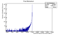
  Figure 1a: The scattered electron total momentum distribution for an incident 11 GeV electron through a LH2 target.
  

• 

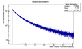
  Figure 1b: The Moller electron total momentum distribution for an incident 11 GeV electron through a LH2 target.

Angular Distribution in the Lab Frame

Momentum distributions in the Center of Mass Frame.

Estimated Momentum Distribution

Performing the relativistic transformation,

For an incoming electron with momentum of 11GeV, we should find the momentum in the center of mass to be around 53 MeV which is confirmed in both the data and the plots.

KEi	Pxi	Pyi	Pzi	xi	yi	z1	KEf	Pxf	Pyf	Pzf	xf	yf	zf	KEm	Pxm	Pym	Pzm	xm	ym	zm
11000	0	0	11000.5	0	0	-510	10999.1	0.433025	-0.858867	10999.6	0	0	-509.276	0.905324	-0.433025	0.858867	0.905366	0	0	-509.276

Changing the code for the total Energy to [math]E=(p_1^2+m_1^2)^{1/2}[/math] in the lab frame gives

Angular Distribution in the Center of Mass Frame

Comparing experimental vs. theoretical for Møller differential cross section 11GeV

Using the equation from [1]

[math]\frac{d\sigma}{d\Omega}=\frac{ e^4 }{8E^2}\left \{\frac{1+cos^4\frac{\theta}{2}}{sin^4\frac{\theta}{2}}+\frac{1+sin^4\frac{\theta}{2}}{cos^4\frac{\theta}{2}}+\frac{2}{sin^2\frac{\theta}{2}cos^2\frac{\theta}{2}} \right \}[/math]

where [math]\alpha=\frac{e^2}{\hbar c}\quad with\quad \hbar = c =1[/math]

This can be simplified to the form

[math]\frac{d\sigma}{d\Omega}=\frac{ \alpha^2 }{4E^2}\frac{ (3+cos^2\theta)^2}{sin^4\theta}[/math]

Plugging in the values expected for a scattering electron:

[math]\alpha ^2=5.3279\times 10^{-5}[/math]

[math]E\approx 53 MeV[/math]

Using unit analysis on the term outside the parantheses, we find that the differential cross section for an electron at this momentum should be around

[math]\frac{5.3279\times 10^{-5}}{4\times 2.81\times 10^{15}eV^2}=4.74\times 10^{-21} eV^{-2}=\frac{4.74\times 10^{-21}}{1eV^2}\times \frac{1\times 10^{18}eV^2 }{1\ GeV^2}=\frac{.0047}{GeV^2}[/math]

Using the conversion of

[math]\frac{1}{1GeV^2}=.3894 mb[/math]

[math]\frac{1\ GeV^{-2}}{.3894\ mb}=\frac{.0047\ GeV^{-2}}{x\ mb}[/math]

The trigonometric function part of the equation comes out to it's minimum of 9 at 90 degrees.

[math]\frac{(3+Cos^2(90))^2}{Sin^4(90)}=9[/math]

We find that the differential cross section scale is [math]\frac{d\sigma}{d\Omega}\approx 1.8\times 10^{-3}mb \times 9=16.2\mu b[/math]

Converting the number of electrons to barns,

[math]L=\frac{i_{scattered}}{\sigma} \approx i_{scattered}\times \rho_{target}\times l_{target}[/math]

where ρ_target is the density of the target material, l_target is the length of the target, and i_scattered is the number of incident particles scattered.

[math]\rho_{target}\times l_{target}=\frac{70.85 kg}{1 m^3}\times \frac{1 mole}{2.02 g} \times \frac{1000g}{1 kg} \times \frac{6\times10^{23} atoms}{1 mole} \times \frac{1m^3}{(100 cm)^3} \times \frac{1 cm}{ } \times \frac{10^{-24} cm^{2}}{barn} =2.10\times 10^{-2} barns[/math]

[math]\frac{1}{\rho_{target}\times l_{target} \times 4\times 10^7}=1.19\times 10^{-6} barns[/math]

Combining these plots, and rescaling the Final Theta in the Center of Mass for micro-barns, we find

Step 2

Replace the LH2 target with an NH3 target and compare with LH2 target.

The Moller Momentum plot for higher momenta run to increase the number of values

LH2 Vs. NH3

[math]L=\frac{870 kg}{1 m^3}\times \frac{1 mole}{17.03 g} \times \frac{1000g}{1 kg} \times \frac{6\times10^{23} atoms}{1 mole} \times \frac{1cm}{100 cm} \times \frac{1 m}{ } \times \frac{10^{-23} m^2}{barn} =2.10\times 10^{-2} barns[/math]

Figure out the offset

Rerunning the GEANT simulation for a target of solo atoms of Carbon 12, with 4¹⁰ incident 11GeV electrons

Density of target material:

C=2.26 g/cm³

NH3=.86g/cm³

LH2=.07g/cm³

Altering the density of LH2 to be .86g/cm³ we find

Comparing this to the theoretical differential cross section:

As shown above

We find that the differential cross section scale is [math]\frac{d\sigma}{d\Omega}\approx 16.2\times 10^{-2}mb=16.2\mu b[/math]

Converting the number of electrons to barns,

[math]L=\frac{i_{scattered}}{\sigma} \approx i_{scattered}\times \rho_{target}\times l_{target}[/math]

where ρ_target is the density of the target material, l_target is the length of the target, and i_scattered is the number of incident particles scattered.

For LH2:

[math]\frac{1}{\rho_{target}\times l_{target} \times 4\times 10^8}=1.19\times 10^{-8} barns=.0119 \mu b[/math]

For Carbon:

[math]\rho_{target}\times l_{target}=\frac{2.26 g}{1 cm^3}\times \frac{1 mole}{12.0107 g} \times \times \frac{6\times10^{23} atoms}{1 mole} \times \frac{1 cm}{ } \times \frac{10^{-24} cm^{2}}{barn} =1.13\times 10^{-1} barns[/math]

[math]\frac{1}{\rho_{target}\times l_{target} \times 4\times 10^8}=2.21\times 10^{-8} barns=.0221 \mu b[/math]

For Ammonia:

[math]\rho_{target}\times l_{target}=\frac{.8 g}{1 cm^3}\times \frac{1 mole}{17 g} \times \frac{6\times10^{23} atoms}{1 mole} \times \frac{1 cm}{ } \times \frac{10^{-24} cm^2}{barn} =2.82\times 10^{-2} barns[/math]

[math]\frac{1}{\rho_{target}\times l_{target} \times 4\times 10^8}=8.87\times 10^{-8} barns=.0887 \mu b[/math]

Combing plots in Root:

new TBrowser();
TH1F *LH2=new TH1F("LH2","LH2",360,90,180);
LH2->Add(MollerThetaCM,1.19e-8);
LH2->Draw();

TH1F *C12=new TH1F("C12","C12",360,90,180);
C12->Add(MollerThetaCM,2.21e-8);
C12->Draw();

TH1F *NH3=new TH1F("NH3","NH3",360,90,180);
NH3->Add(MollerThetaCM,8.87e-8);
NH3->Draw();
LH2->Draw("same");
C12->Draw("same");
Theory->Draw("same");

Step 3

Determine impact of Solenoid magnet on Moller events

Papers used

[1]Farrukh Azfar's Derivation of Moller Scattering

File:FarrukAzfarMollerScatter.pdf

A polarized target for the CLAS detector

File:PHY02-33.pdf

An investigation of the spin structure of the proton in deep inelastic scattering of polarized muons on polarized protons

File:1819.pdf

QED Radiative Corrections to Low-Energy Moller and Bhabha Scattering

http://arxiv.org/abs/1602.07609

Moller Track Reconstruction

DV_MollerTrackRecon

EG12