DV MollerTrackRecon

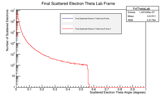
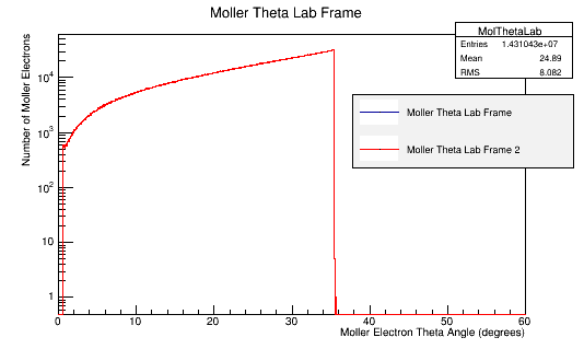
Moller Lund

LUND file with Moller events (with origin of coordinates occurring at each event)

2       1       1       1       1       0       0.000563654     3.53715 0       6.2002
1 -1 1 11 0 0 0.69 -2.4999 10993.7998 10993.80 0.000511 0 0 0
2 -1 1 11 0 0 -0.69 2.4999 6.5852 7.08 0.000511 0 0 0

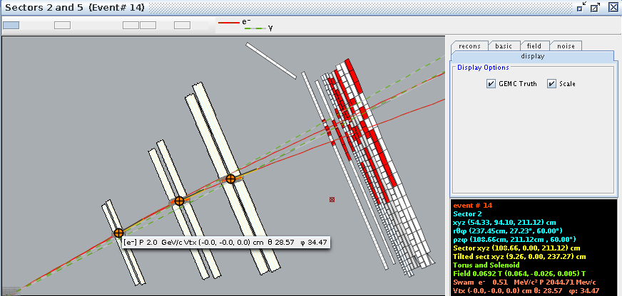
From a GEMC run WITH the Solenoid ced is used to obtain the information from the eg12_rec.ev file.

We take the phi angle from the Generated Event momentum as the initial phi angle. The obtain the final phi angle, we can look at the final position of the electron with in the drift chambers.

Examining the position from Timer Based Tracking, we can see that after rotations about first the y-axis, then the z-axis transforms from the detector frame of reference to the lab frame of reference.

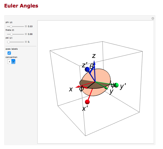
Euler Angles

We can use the Euler angles to perform the rotations.

For the rotation about the y axis.

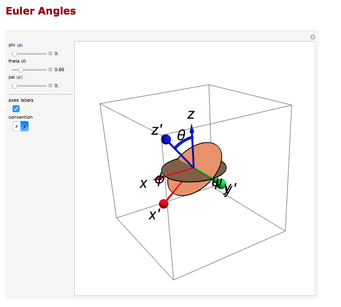
And the rotation about the z axis.

Transformation Matrix

The Euler angles can be applied using a transformation matrix

[math]\left( \begin{array}{ccc} \cos (\theta ) & 0 & -\sin (\theta ) \\ 0 & 1 & 0 \\ \sin (\theta ) & 0 & \cos (\theta ) \\ \end{array} \right).\left( \begin{array}{c} x \\ y \\ z \\ \end{array} \right)[/math]

[math]=\left( \begin{array}{c} x \cos (\theta )-z \sin (\theta ) \\ y \\ z \cos (\theta )+x \sin (\theta ) \\ \end{array} \right)[/math]

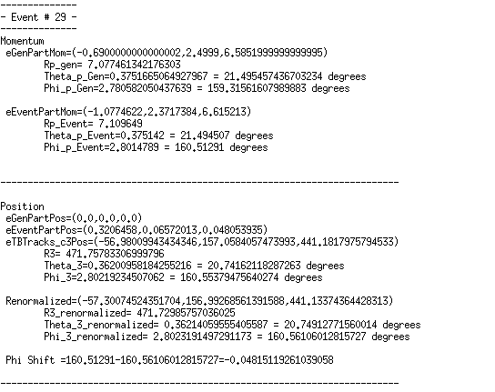
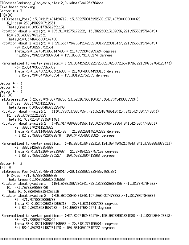
For event #29, in sector 3, the location of the first interaction is given by

Converting -25 degrees to radians, [math]\theta =-0.436332[/math] which is the rotation the detectors are rotated from the y axis.

[math]\left( \begin{array}{ccc} \cos (\theta ) & 0 & -\sin (\theta ) \\ 0 & 1 & 0 \\ \sin (\theta ) & 0 & \cos (\theta ) \\ \end{array} \right).\left( \begin{array}{c} -15.76 \\ 0 \\ 237.43 \\ \end{array} \right)[/math]

[math]=\left( \begin{array}{c} 86.0588 \\ 0. \\ 221.845 \\ \end{array} \right)[/math]

Finding [math]\phi =\frac{120\ 2 \pi }{360};[/math] since "sector -1" =3-1=2*60=120 degrees

[math]\left( \begin{array}{ccc} \cos (\phi ) & -\sin (\phi ) & 0 \\ \sin (\phi ) & \cos (\phi ) & 0 \\ 0 & 0 & 1 \\ \end{array} \right).\left( \begin{array}{c} 86.0588 \\ 0. \\ 221.845 \\ \end{array} \right)[/math]

[math]\left( \begin{array}{c} -43.0294 \\ 74.5291 \\ 221.845 \\ \end{array} \right)[/math]

This shows how the coordinates are transformed and explains the validity of using the TBTracking information to obtain a phi angle in the lab frame.

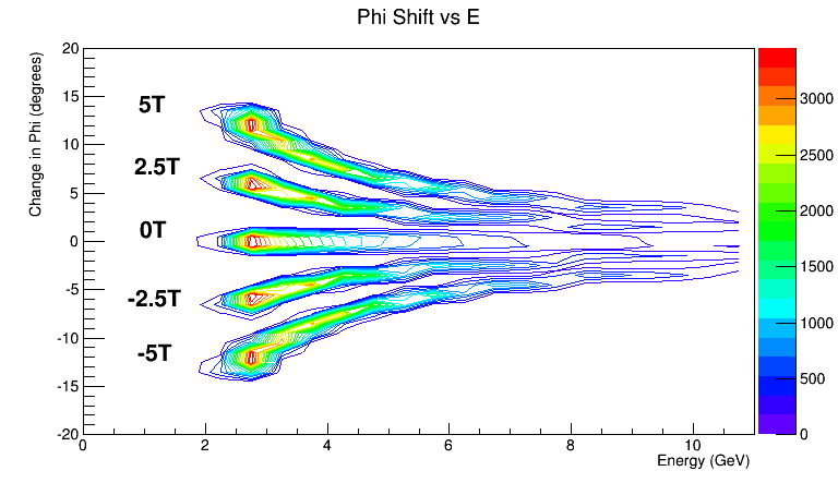
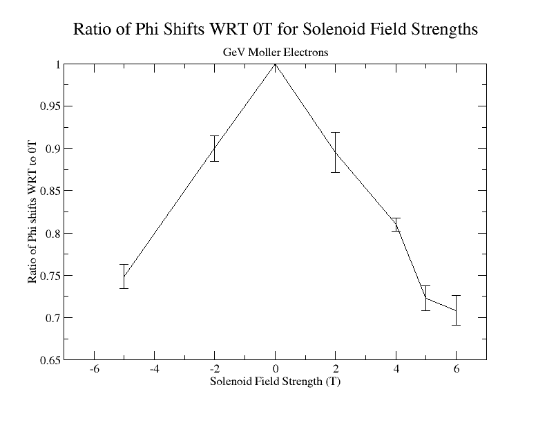
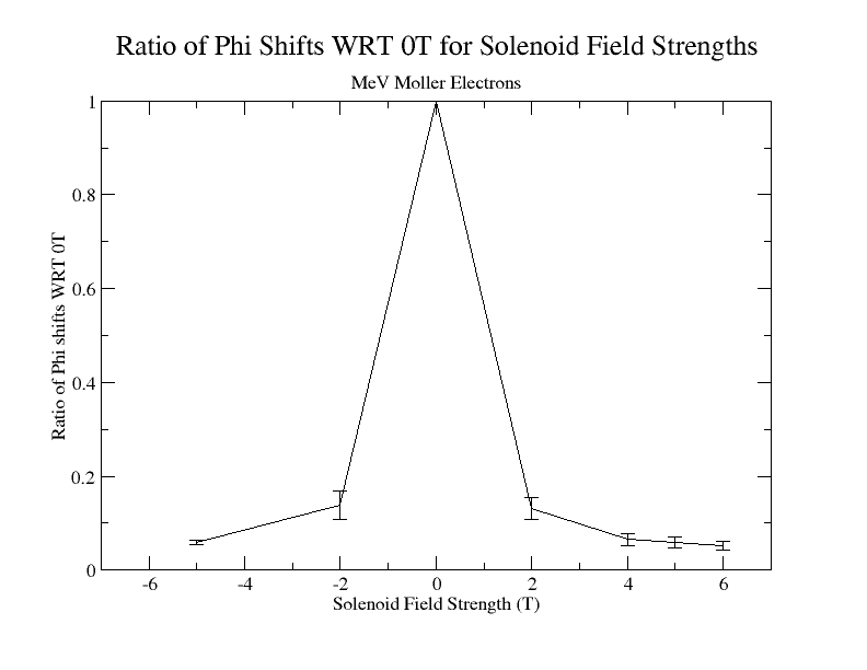
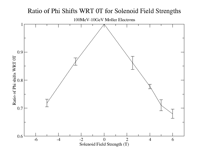
Phi shifts

gcard to generate electrons.

 <option name="BEAM_P"   value="e-, 6.0*GeV, 30.0*deg, 10*deg">
 <option name="SPREAD_P" value="5.5*GeV, 25*deg, 180*deg">

Cross-section

Calculations of 4-momentum components

DV_Calculations_of_4-momentum_components

Summary of 4-momentum calculations

[math]For\ 0 \ge \phi \ge \frac{-\pi}{2}\ Radians[/math]

x=POSITIVE

y=NEGATIVE

[math]For\ 0 \le \phi \le \frac{\pi}{2}\ Radians[/math]

x=POSITIVE

y=POSITIVE

[math]For\ \frac{-\pi}{2} \ge \phi \ge -\pi\ Radians[/math]

x=NEGATIVE

y=NEGATIVE

[math]For\ \frac{\pi}{2} \le \phi \le \pi\ Radians[/math]

x=NEGATIVE

y=POSITIVE

4 momentum calculations for different frames of reference

Electron Initial Lab Frame	Moller electron Initial Lab Frame	Moller electron Final Lab Frame	Moller electron Center of Mass Frame	Electron Center of Mass Frame	Electron Final Lab Frame
[math]p_{1}\equiv 11000 MeV[/math]	[math]p_{2}\equiv 0[/math]	[math]p_{2}'\equiv INPUT[/math]	[math]p_{2}^*=\sqrt{E_{2}^{*2}-m^2}[/math]	[math]p_{1}^*=\sqrt{E_{2}^{*2}-m^2}[/math]	[math]p_{1}'=\sqrt{E_{1}^{'\ 2}-m^2}[/math]
[math]\theta_{1}\equiv 0[/math]	[math]\theta_{2}\equiv 0[/math]	[math]\theta_{2}'\equiv INPUT[/math]	[math]\theta_{2}^*=\arccos \left(\frac{p_{2(z)}^*}{p_2^*} \right)[/math]	[math]\theta_{1}^*=\pi-\theta_{2}^*[/math]	[math]\theta_{1}'= \arccos \left(\frac{p_{1(z)}'}{p_{1}'} \right)[/math]
[math]E_{1}=\sqrt{p_1^2+m^2}[/math]	[math]E_{2}\equiv m[/math]	[math]E_{2}'=\sqrt{p_{2}^{'\ 2}+m^2}[/math]	[math]E_{2}^*=\sqrt{\frac{m(m+E_1)}{2}}[/math]	[math]E_{1}^*=\sqrt{\frac{m(m+E_1)}{2}}[/math]	[math]E_{1}'\equiv E'-E_{2}'[/math]
[math]p_{1(x)}\equiv 0[/math]	[math]p_{2(x)}\equiv 0[/math]	[math]p_{2(x)}'=\sqrt{p_{2}^{'\ 2}-p_{2(z)}^{'\ 2}} cos(\phi '_2)[/math]	[math]p_{2(x)}^*\equiv p_{2(x)}'[/math]	[math]p_{1(x)}^*\equiv-p_{2(x)}^*[/math]	[math]p_{1(x)}'\equiv p_{1(x)}^*[/math]
[math]p_{1(y)}\equiv 0[/math]	[math]p_{2(y)}\equiv 0[/math]	[math]p_{2(y)}'=\sqrt{p_{2}^{'\ 2}-p_{2(x)}^{'\ 2}-p_{2(z)}^{'\ 2}}[/math]	[math]p_{2(y)}^*\equiv p_{2(y)}'[/math]	[math]p_{1(y)}^*\equiv -p_{2(y)}^*[/math]	[math]p_{1(y)}'\equiv p_{2(y)}^*[/math]
[math]p_{1(z)}\equiv p_1[/math]	[math]p_{2(z)}\equiv 0[/math]	[math]p_{2(z)}'\equiv p_{2}'\ cos(\theta'_2)[/math]	[math]p_{2(z)}^*=-\sqrt{p_{2}^{*\ 2}-p_{2(x)}^{*\ 2}-p_{2(y)}^{*\ 2}}[/math]	[math]p_{1(z)}^*\equiv -p_{2(z)}^*[/math]	[math]p_{1(z)}'=\sqrt{p_{1}^{'\ 2}-p_{(1(x)}^{'\ 2}-p_{1(y)}^{'\ 2}}[/math]

[[File:]][[File:]]

[[File:]][[File:]]

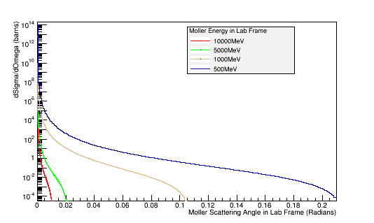
Differential Cross Section

Moller Differential Cross Section

Using the equation from [1]

[math]\frac{d\sigma}{d\Omega '_1}=\frac{ e^4 }{8E^{*2}}\left \{\frac{1+cos^4(\frac{\theta^*}{2})}{sin^4(\frac{\theta^*}{2})}+\frac{1+sin^4(\frac{\theta^*}{2})}{cos^4(\frac{\theta^*}{2})}+\frac{2}{sin^2(\frac{\theta^*}{2})cos^2(\frac{\theta^*}{2})} \right \}[/math]

[math]where\ \alpha=\frac{e^2}{\hbar c}\quad with\quad \hbar = c =1\ and\ \theta^*=\theta^*_1=\theta^*_2[/math]

This can be simplified to the form

[math]\frac{d\sigma}{d\Omega '_1}=\frac{ \alpha^2 }{4E^{*2}}\frac{ (3+cos^2\theta^*)^2}{sin^4\theta^*}[/math]

Plugging in the values expected for 2 scattering electrons:

[math]\alpha ^2=5.3279\times 10^{-5}[/math]

[math]E^*\approx 106.031 MeV[/math]

Using unit analysis on the term outside the parantheses, we find that the differential cross section for an electron at this momentum should be around

[math]\frac{5.3279\times 10^{-5}}{4\times 1.124\times 10^{16}eV^2}=1.18\times 10^{-21} eV^{-2}=\frac{1.18\times 10^{-21}}{1eV^2}\times \frac{1\times 10^{18} }{1\times 10^{18}}=\frac{.0012}{GeV^2}[/math]

Using the conversion of

[math]\frac{1}{1GeV^2}=.3894 mb[/math]

[math]\frac{.0012}{1GeV^2}=\frac{.0012}{1}\frac{1}{1GeV^2}=.0012\times .3894 mb=.467\times 10^{-3}mb[/math]

We find that the differential cross section scale is [math]\frac{d\sigma}{d\Omega}\approx .5\times 10^{-3}mb=.5\mu b[/math]

CM to Lab Frame

We can substitute in for [math]\theta[/math]

[math]\frac{d\sigma}{d\Omega '_1}=\frac{ \alpha^2 }{4E^{*2}}\frac{ (3+cos^2\theta^*)^2}{sin^4\theta^*}[/math]

[math]\frac{d\sigma}{d\Omega '_1}=\frac{ \alpha^2 }{4E^{*2}}\frac{ (3+cos^2\theta^*)^2}{sin(\theta^*)sin(\theta^*)sin(\theta^*)sin(\theta^*)}[/math]

Using,

[math]sin(\theta^*)=sin(\theta_{2}^*)=\frac{p_{2}'}{p_{2}^*}\ sin \left( \theta_{2}'\right)[/math]

[math]\frac{d\sigma}{d\Omega '_1}=\frac{ \alpha^2 }{4E^{*2}}\frac{ (3+cos^2\theta^*)^2}{\frac{p_{2}'}{p_{2}^*}\ sin \left( \theta_{2}'\right)\frac{p_{2}'}{p_{2}^*}\ sin \left( \theta_{2}'\right)\frac{p_{2}'}{p_{2}^*}\ sin \left( \theta_{2}'\right)\frac{p_{2}'}{p_{2}^*}\ sin \left( \theta_{2}'\right)}[/math]

[math]\frac{d\sigma}{d\Omega '_1}=\frac{ \alpha^2 p_{2}^{*4}}{4E^{*2}p_{2}'^4}\frac{ (3+cos^2\theta^*)^2}{sin^4 \left( \theta_{2}'\right)}[/math]

Now, using the trigometric identity,

[math]sin^2 t+cos^2 t=1\Longrightarrow cos^2(\theta^*)=1-sin^2(\theta^*)[/math]

[math]\frac{d\sigma}{d\Omega '_1}=\frac{ \alpha^2 p_{2}^{*4}}{4E^{*2}p_{2}'^4}\frac{ (3+1-sin^2(\theta^*))^2}{sin^4 \left( \theta_{2}'\right)}[/math]

[math]\frac{d\sigma}{d\Omega '_1}=\frac{ \alpha^2 p_{2}^{*4}}{4E^{*2}p_{2}'^4}\frac{ (4-sin(\theta^*)sin(\theta^*))^2}{sin^4 \left( \theta_{2}'\right)}[/math]

[math]\frac{d\sigma}{d\Omega '_1}=\frac{ \alpha^2 p_{2}^{*4}}{4E^{*2}p_{2}'^4}\frac{ (4-\frac{p_{2}'}{p_{2}^*}\ sin \left( \theta_{2}'\right)\frac{p_{2}'}{p_{2}^*}\ sin \left( \theta_{2}'\right))^2}{sin^4 \left( \theta_{2}'\right)}[/math]

[math]\frac{d\sigma}{d\Omega '_1}=\frac{ \alpha^2 p_{2}^{*4}}{4E^{*2}p_{2}'^4}\frac{ (4-\frac{p_{2}^{'2}}{p_{2}^{*2}}\ sin^2 \left( \theta_{2}'\right))^2}{sin^4 \left( \theta_{2}'\right)}[/math]

[math]\frac{d\sigma}{d\Omega '_1}=\frac{ \alpha^2 p_{2}^{*4}}{4E^{*2}p_{2}'^4}\frac{ (16-8\frac{p_{2}^{'2}}{p_{2}^{*2}}\ sin^2 \left( \theta_{2}'\right)+\frac{p_{2}^{'4}}{p_{2}^{*4}}\ sin^4 \left( \theta_{2}'\right))}{sin^4 \left( \theta_{2}'\right)}[/math]

Substituting,

[math]p_{2}^*=\sqrt{E_{2}^{*2}-m^2}[/math]

[math]\frac{d\sigma}{d\Omega '_1}=\frac{ \alpha^2 (\sqrt{E_{2}^{*2}-m^2})^4}{4E^{*2}p_{2}'^4}\frac{ (16-8\frac{p_{2}^{'2}}{p_{2}^{*2}}\ sin^2 \left( \theta_{2}'\right)+\frac{p_{2}^{'4}}{p_{2}^{*4}}\ sin^4 \left( \theta_{2}'\right))}{sin^4 \left( \theta_{2}'\right)}[/math]

[math]\frac{d\sigma}{d\Omega '_1}=\frac{ \alpha^2 (E_{2}^{*2}-m^2)^2}{4E^{*2}p_{2}'^4}\frac{ (16-8\frac{p_{2}^{'2}}{p_{2}^{*2}}\ sin^2 \left( \theta_{2}'\right)+\frac{p_{2}^{'4}}{p_{2}^{*4}}\ sin^4 \left( \theta_{2}'\right))}{sin^4 \left( \theta_{2}'\right)}[/math]

Substituting in for m, E₂^*,and E^* [math]\alpha^2=5.3279\times 10^{-5}[/math]

[math]\frac{d\sigma}{d\Omega '_1}=(\frac{ 5.3279\times 10^{-5}( ((53.015MeV)^{2}-(.511MeV)^2)^2}{4\times (106.031MeV)^{2}p_{2}'^4}\frac{ (16-8\frac{p_{2}^{'2}}{p_{2}^{*2}}\ sin^2 \left( \theta_{2}'\right)+\frac{p_{2}^{'4}}{p_{2}^{*4}}\ sin^4 \left( \theta_{2}'\right))}{sin^4 \left( \theta_{2}'\right)}[/math]

[math]\frac{d\sigma}{d\Omega '_1}=\frac{9.357\times 10^9eV^2}{p_{2}^{'4}}\frac{ (16-8\frac{p_{2}^{'2}}{p_{2}^{*2}}\ sin^2 \left( \theta_{2}'\right)+\frac{p_{2}^{'4}}{p_{2}^{*4}}\ sin^4 \left( \theta_{2}'\right))}{sin^4 \left( \theta_{2}'\right)}[/math]

Different p₂¹ Values

Using the conversion of

[math]\frac{1}{1GeV^2}=.3894 mb[/math]

[math]\sigma=\int d\sigma=\int \frac{d\sigma}{d\Omega_2'}d\Omega[/math]

The range of the detector is considered to be [math] .10 \le \theta \le .87[/math],[math]-\pi \le \phi \le \pi[/math]

[math]\sigma=\int_{ .611}^{2.531} \int_{-\pi}^{\pi} \frac{d\sigma}{d\Omega_2'}sin\theta \,d\theta \, d\phi [/math]

[math]\sigma=2\pi \int_{.611}^{2.531} \frac{d\sigma}{d\Omega_2'} sin\theta \,d\theta [/math]

[math]\sigma=2\pi (1.638)\frac{d\sigma}{d\Omega_2'} [/math]

[math]\sigma=(10.294) \frac{d\sigma}{d\Omega_2'} [/math]

Differential Cross Section Scale for Different p₂¹ Values

[math]p_{2}'(MeV)[/math]	[math]\frac{d\sigma}{d\Omega_{2}^'}(eV^{-2})[/math]	[math]\frac{d\sigma}{d\Omega_{2}^'}(GeV^{-2})[/math]	[math]\frac{d\sigma}{d\Omega_{2}^'}(mb)[/math]	[math]\frac{d\sigma}{d\Omega_{2}^'}(b)[/math]	[math]\sigma(b)[/math]
[math]10000[/math]	[math]9.357\times 10^{-11}[/math]	[math]9.357\times 10^{7}[/math]	[math]3.644\times 10^{7}[/math]	[math]3.644\times 10^{4}[/math]	[math]3.751\times 10^{5}[/math]
[math]5000 [/math]	[math]3.743\times 10^{-10}[/math]	[math]3.743\times 10^{8}[/math]	[math]1.458\times 10^{8}[/math]	[math]1.458\times 10^{5}[/math]	[math]1.501\times 10^{6}[/math]
[math]1000 [/math]	[math]9.357\times 10^{-9}[/math]	[math]9.357\times 10^{9}[/math]	[math]3.644\times 10^{9}[/math]	[math]3.644\times 10^{6}[/math]	[math]3.751\times 10^{7}[/math]
[math]500[/math]	[math]3.743\times 10^{-8}[/math]	[math]3.743\times 10^{10}[/math]	[math]1.458\times 10^{10}[/math]	[math]1.458\times 10^{7}[/math]	[math]1.501\times 10^{8}[/math]

Substituting for Moller range and energies

Converting the number of electrons to barns,

[math]\frac{d\sigma}{d\Omega_{2}'}=\frac{dN}{\mathcal L d\Omega}[/math]

[math]\mathcal L=\Phi \rho l[/math]

[math]\Longrightarrow N=\sigma \Phi \rho l[/math]

where ρ_target is the density of the target material, l_target is the length of the target, and N is the number of incident particles scattered.

[math]\mathcal L=\frac{.86g}{1 cm^3}\times \frac{(100cm)^3}{1m^3} \times \frac{1 kg}{1000 g}\times \left[ \left(.75 \frac{1 mole}{1.01 g} \times \frac{1000g}{1 kg} \right)+\left(.25 \frac{1 mole}{14.01 g} \times \frac{1000g}{1 kg} \right)\right] \times \frac{6.022\times10^{23}particles}{1 mole} \times \frac{1cm}{100 cm} \times \frac{1 m}{ } \times \frac{10^{-28} m^2}{barn} [/math]

[math]\mathcal L=\frac{860kg}{1 m^3}\times \left[ \left(\frac{742.574 mole}{kg} \right)+\left(\frac{17.844 mole}{1 kg} \right)\right] \times \frac{6.022\times 10^{-7}\ particles\cdot m^3}{1 mole\cdot barn} [/math]

[math]\mathcal L=\frac{5.170\times 10^{-4}kg\cdot particles}{1 mole\cdot barn} \left(\frac{760.418 mole}{kg} \right)[/math]

[math]\mathcal L=\frac{.394\ particles}{1 barn} [/math]

[math]\Longrightarrow N=\sigma \frac{.394\ particles}{1 barn}[/math]

Number of electrons from Moller electron Momentum

[math]p_2^{'}(MeV/c)[/math]	[math]\sigma(b)[/math]	[math]Number of electrons[/math]
[math]\equiv 10000[/math]	[math]3.751\times 10^{5}[/math]	[math]\approx 1.478\times 10^5[/math]
[math]\equiv 5000 [/math]	[math]1.501\times 10^{6}[/math]	[math]\approx5.914\times 10^5[/math]
[math]\equiv 1000 [/math]	[math]3.751\times 10^{7}[/math]	[math]\approx 1.478\times 10^7[/math]
[math]\equiv 500[/math]	[math]1.501\times 10^{8}[/math]	[math]\approx 5.914\times 10^7[/math]