DV MollerTrackRecon

Moller Lund

LUND file with Moller events (with origin of coordinates occurring at each event)

2       1       1       1       1       0       0.000563654     3.53715 0       6.2002
1 -1 1 11 0 0 0.69 -2.4999 10993.7998 10993.80 0.000511 0 0 0
2 -1 1 11 0 0 -0.69 2.4999 6.5852 7.08 0.000511 0 0 0

From a GEMC run WITH the Solenoid ced is used to obtain the information from the eg12_rec.ev file.

We take the phi angle from the Generated Event momentum as the initial phi angle. The obtain the final phi angle, we can look at the final position of the electron with in the drift chambers.

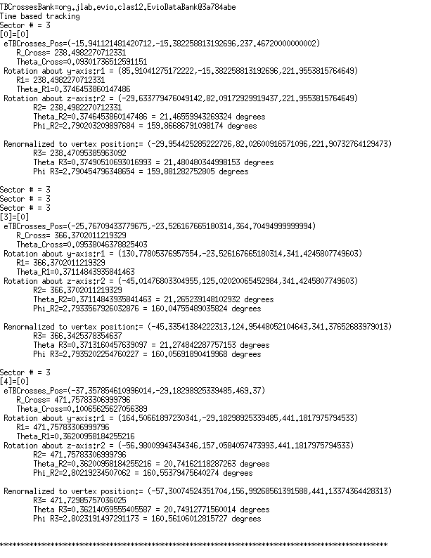
Examining the position from Timer Based Tracking, we can see that after rotations about first the y-axis, then the z-axis transforms from the detector frame of reference to the lab frame of reference.

Euler Angles

We can use the Euler angles to perform the rotations.

For the rotation about the y axis.

And the rotation about the z axis.

Transformation Matrix

The Euler angles can be applied using a transformation matrix

[math]\left( \begin{array}{ccc} \cos (\theta ) & 0 & -\sin (\theta ) \\ 0 & 1 & 0 \\ \sin (\theta ) & 0 & \cos (\theta ) \\ \end{array} \right).\left( \begin{array}{c} x \\ y \\ z \\ \end{array} \right)[/math]

[math]=\left( \begin{array}{c} x \cos (\theta )-z \sin (\theta ) \\ y \\ z \cos (\theta )+x \sin (\theta ) \\ \end{array} \right)[/math]

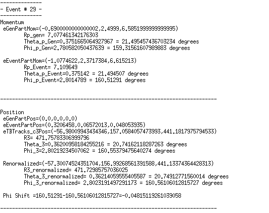
For event #29, in sector 3, the location of the first interaction is given by

Converting -25 degrees to radians, [math]\theta =-0.436332[/math] which is the rotation the detectors are rotated from the y axis.

[math]\left( \begin{array}{ccc} \cos (\theta ) & 0 & -\sin (\theta ) \\ 0 & 1 & 0 \\ \sin (\theta ) & 0 & \cos (\theta ) \\ \end{array} \right).\left( \begin{array}{c} -15.76 \\ 0 \\ 237.43 \\ \end{array} \right)[/math]

[math]=\left( \begin{array}{c} 86.0588 \\ 0. \\ 221.845 \\ \end{array} \right)[/math]

Finding [math]\phi =\frac{120\ 2 \pi }{360};[/math] since "sector -1" =3-1=2*60=120 degrees

[math]\left( \begin{array}{ccc} \cos (\phi ) & -\sin (\phi ) & 0 \\ \sin (\phi ) & \cos (\phi ) & 0 \\ 0 & 0 & 1 \\ \end{array} \right).\left( \begin{array}{c} 86.0588 \\ 0. \\ 221.845 \\ \end{array} \right)[/math]

[math]\left( \begin{array}{c} -43.0294 \\ 74.5291 \\ 221.845 \\ \end{array} \right)[/math]

This shows how the coordinates are transformed and explains the validity of using the TBTracking information to obtain a phi angle in the lab frame.

Phi shifts

gcard to generate electrons.

 <option name="BEAM_P"   value="e-, 6.0*GeV, 30.0*deg, 10*deg">
 <option name="SPREAD_P" value="5.5*GeV, 25*deg, 180*deg">

Cross-section

Previous attempts

Calculations of 4-momentum components (Trial 4)

Setup

Since we want to run for a evenly spaced energy range for Moller electrons, we will need to use some of the scattered electrons to help cover this range. A Moller scattering data file of 1E7 events has no Moller electrons with momentum over 5500 MeV. Since momentum is conserved, and the data is verified kinematicly verified, we cannot simply "switch" the data. This data can be altered to have a certain number of different phi values for each energy to match the Moller cross section. This data can then be written to a LUND file, and compared to the previous calculations which did not factor in loss of initial energy.

Prepare Data

Using the existing Moller scattering data from a GEANT simulation of 4E7 incident electrons, a file of just scattered momentum components can be constructed using:

awk '{print $9, $10, $11, $16, $17, $18}' MollerScattering_NH3_Large.dat > Just_Scattered_Momentum.dat

Transfer to CM Frame

Reading in the data from the dat file, we use a C++ program to read the momentum components for the Scattered and Moller electrons into 4-momentum vectors defined as the Lab_final frame of reference.

Performing a Lorentz boost to a Center of Mass frame for the two 4-vectors from the Lab_final frame of reference, we move to a frame where the energies are equal and the momentum are equal but opposite.

Relativistic Kinematics

For Moller Electron energies above 500 MeV, in the Lab frame, histograms of momentum, and theta as well as a 2-D histogram of Energy vs. Theta for the Moller Electron in the CM frame will be filled.

Using the histogram for Theta in the CM frame, we can determine the relative number of events that occur at a given angle. This information will be used to keep the relative number of particles having the same Theta angle, but multiple Psi angles to evenly cover the detector area

Run for Necessary Amount to match Cross Section

Using the above plot for the target material, we can find the relative amount that each Theta angle should observe for this process which gives a known Moller differential cross section.

Theta (degrees)	Number of events
90	5
100	5
110	6
120	8
130	12
135	20
140	28
142	30
144	40
146	45
148	55
150	70
152	80
154	100

We can set up conditional statements to check what range the Theta angle falls in, then by dividing

[math]\Delta \phi=\frac {2\pi}{number\ of\ events}[/math]

we should find the change in phi needed to give an evenly distributed distribution around the xy plane for a given Theta angle.

Alter Phi Angles

Using the fact that

[math]\cos{\phi} \equiv \frac{p_x}{\sqrt{p^2-p_z^2}}[/math]

[math]\Longrightarrow \sqrt{p^2-p_z^2}=\frac{p_x}{\cos{\phi}}=constant[/math]

We can simply use the expression

[math]\frac{p_x}{\cos{\phi}}=\frac{p_x'}{cos{\left(\phi+\delta \phi\right)}}[/math]

[math]\Longrightarrow p_x'=\frac{p_x \times \cos{\left(\phi+\delta \phi\right)}}{\cos{\phi}}[/math]

Then, using

[math]\sqrt{p^2-p_z^2}=\sqrt{p_x^2+p_y^2}[/math]

[math]\Longrightarrow p_y'=\sqrt{p^2-p_z^2-p_x^{'2}}[/math]

Starting with a data file of momentum components constructed using awk as described above

A program was written to rotate the phi angle as described above. The changing x and y components for this distribution can be seen with

Lastly a LUND file was written that was 643360680 lines in length, which equates to 214453560 entries. This was divided into 8579 file parts of 75000 each. The first set from the original data set is shown below. To make sure the full 2 pi is covered, the rotation starts in the 1st quadrant.

split -a 4 -d -l 75000 Extra_Phi.LUND Phi_Parts_

---

Back to Recon

Differential Cross Section

Variables used in Elastic Scattering

Variables Used in Elastic Scattering

Scattering Cross Section

Scattering Cross Section

old work