|
|
| Line 138: |
Line 138: |
| | | | |
| | =Cross-section Area= | | =Cross-section Area= |
| | + | |
| | + | ==Moller electron Lab Frame== |
| | + | Finding the correct kinematic values starting from knowing the momentum of the Moller (m) electron in the Lab frame, |
| | + | |
| | + | |
| | + | |
| | + | <center>Using <math>\theta=\arccos(\frac{P_{z(m) Lab}}{P_{(m)Lab}})</math></center> |
| | + | |
| | + | {| class="wikitable" align="center" |
| | + | | style="background: gray" | <math>\Longrightarrow {P_{z(m) Lab}=P_{(m)Lab}\cos(\theta)}</math> |
| | + | |} |
| | + | |
| | + | |
| | + | |
| | + | <center>Similarly, <math>\phi=\arccos(\frac{P_{x(m) Lab}}{P_{xy(m) Lab}})</math></center> |
| | + | |
| | + | |
| | + | <center>where <math>P_{xy(m) Lab}=\sqrt{P_{x(m) Lab}^2+P_{y(m)Lab}^2}</math></center> |
| | + | |
| | + | |
| | + | <center><math>P_{xy(m) Lab}=(P_{x(m) Lab}^2+P_{y(m) Lab}^2)^2</math></center> |
| | + | |
| | + | |
| | + | <center>and using <math>P_{(m)Lab}^2=P_{x(m) Lab}^2+P_{y(m) Lab}^2+P_{z(m) Lab}^2</math></center> |
| | + | |
| | + | |
| | + | <center>this gives <math>P_{(m)Lab}^2=P_{xy(m) Lab}^2+P_{z(m) Lab}^2</math></center> |
| | + | |
| | + | |
| | + | <center><math>\Longrightarrow P_{(m)Lab}^2-P_{z(m) Lab}^2=P_{xy(m) Lab}^2</math></center> |
| | + | |
| | + | |
| | + | <center><math>\Longrightarrow P_{xy(m) Lab}=\sqrt{P_{(m)Lab}^2-P_{z(m) Lab}^2}</math></center> |
| | + | |
| | + | |
| | + | <center>which gives<math>\phi = \arccos(\frac{P_{x(m) Lab}}{\sqrt{P_{(m)Lab}^2-P_{z(m) Lab}^2}})</math></center> |
| | + | |
| | + | {| class="wikitable" align="center" |
| | + | | style="background: gray" | <math>\Longrightarrow P_{x(m) Lab}=\sqrt{P_{(m)Lab}^2-P_{z(m) Lab}^2} \cos(\phi)</math> |
| | + | |} |
| | + | |
| | + | |
| | + | <center>Similarly, using <math>P_{(m)Lab}^2=P_{x(m) Lab}^2+P_{y(m) Lab}^2+P_{z(m) Lab}^2</math></center> |
| | + | |
| | + | |
| | + | <center><math>\Longrightarrow P_{(m)Lab}^2-P_{x(m) Lab}^2-P_{z(m) Lab}^2=P_{y(m) Lab}^2</math></center> |
| | + | |
| | + | {| class="wikitable" align="center" |
| | + | | style="background: gray" | <math>P_{y(m) Lab}=\sqrt{P_{(m)Lab}^2-P_{x(m) Lab}^2-P_{z(m) Lab}^2}</math> |
| | + | |} |
| | + | |
| | + | |
| | + | |
| | + | Relativistically, the x and y components remain the same in the conversion from the Lab frame to the Center of Mass frame, since the direction of motion is only in the z direction. |
| | + | |
| | + | |
| | + | |
| | + | {| class="wikitable" align="center" |
| | + | | style="background: gray" | <math>P_{x(m) CM}\Leftrightarrow P_{x(m) Lab}</math> |
| | + | |} |
| | + | |
| | + | |
| | + | {| class="wikitable" align="center" |
| | + | | style="background: gray" | <math>P_{y(m) CM}\Leftrightarrow P_{y(m) Lab}</math> |
| | + | |} |
| | + | |
| | + | |
| | + | |
| | + | {| class="wikitable" align="center" |
| | + | | style="background: gray" | <math>P_{z(m) CM}=\sqrt{P_{(m)CM}^2-P_{x(m) CM}^2-P_{y(m) CM}^2}</math> |
| | + | |} |
| | + | |
| | ==Center of Mass Energy== | | ==Center of Mass Energy== |
| | Using the definition | | Using the definition |
| Line 335: |
Line 407: |
| | |} | | |} |
| | | | |
| − | ==Moller electron Lab Frame==
| |
| − | Finding the correct kinematic values starting from knowing the momentum of the Moller (m) electron in the Lab frame,
| |
| − |
| |
| − |
| |
| − |
| |
| − | <center>Using <math>\theta=\arccos(\frac{P_{z(m) Lab}}{P_{(m)Lab}})</math></center>
| |
| − |
| |
| − | {| class="wikitable" align="center"
| |
| − | | style="background: gray" | <math>\Longrightarrow {P_{z(m) Lab}=P_{(m)Lab}\cos(\theta)}</math>
| |
| − | |}
| |
| − |
| |
| − |
| |
| − |
| |
| − | <center>Similarly, <math>\phi=\arccos(\frac{P_{x(m) Lab}}{P_{xy(m) Lab}})</math></center>
| |
| − |
| |
| − |
| |
| − | <center>where <math>P_{xy(m) Lab}=\sqrt{P_{x(m) Lab}^2+P_{y(m)Lab}^2}</math></center>
| |
| − |
| |
| − |
| |
| − | <center><math>P_{xy(m) Lab}=(P_{x(m) Lab}^2+P_{y(m) Lab}^2)^2</math></center>
| |
| − |
| |
| − |
| |
| − | <center>and using <math>P_{(m)Lab}^2=P_{x(m) Lab}^2+P_{y(m) Lab}^2+P_{z(m) Lab}^2</math></center>
| |
| − |
| |
| − |
| |
| − | <center>this gives <math>P_{(m)Lab}^2=P_{xy(m) Lab}^2+P_{z(m) Lab}^2</math></center>
| |
| − |
| |
| − |
| |
| − | <center><math>\Longrightarrow P_{(m)Lab}^2-P_{z(m) Lab}^2=P_{xy(m) Lab}^2</math></center>
| |
| − |
| |
| − |
| |
| − | <center><math>\Longrightarrow P_{xy(m) Lab}=\sqrt{P_{(m)Lab}^2-P_{z(m) Lab}^2}</math></center>
| |
| − |
| |
| − |
| |
| − | <center>which gives<math>\phi = \arccos(\frac{P_{x(m) Lab}}{\sqrt{P_{(m)Lab}^2-P_{z(m) Lab}^2}})</math></center>
| |
| − |
| |
| − | {| class="wikitable" align="center"
| |
| − | | style="background: gray" | <math>\Longrightarrow P_{x(m) Lab}=\sqrt{P_{(m)Lab}^2-P_{z(m) Lab}^2} \cos(\phi)</math>
| |
| − | |}
| |
| − |
| |
| − |
| |
| − | <center>Similarly, using <math>P_{(m)Lab}^2=P_{x(m) Lab}^2+P_{y(m) Lab}^2+P_{z(m) Lab}^2</math></center>
| |
| − |
| |
| − |
| |
| − | <center><math>\Longrightarrow P_{(m)Lab}^2-P_{x(m) Lab}^2-P_{z(m) Lab}^2=P_{y(m) Lab}^2</math></center>
| |
| − |
| |
| − | {| class="wikitable" align="center"
| |
| − | | style="background: gray" | <math>P_{y(m) Lab}=\sqrt{P_{(m)Lab}^2-P_{x(m) Lab}^2-P_{z(m) Lab}^2}</math>
| |
| − | |}
| |
| − |
| |
| − |
| |
| − |
| |
| − | Relativistically, the x and y components remain the same in the conversion from the Lab frame to the Center of Mass frame, since the direction of motion is only in the z direction.
| |
| − |
| |
| − |
| |
| − |
| |
| − | {| class="wikitable" align="center"
| |
| − | | style="background: gray" | <math>P_{x(m) CM}\Leftrightarrow P_{x(m) Lab}</math>
| |
| − | |}
| |
| − |
| |
| − |
| |
| − | {| class="wikitable" align="center"
| |
| − | | style="background: gray" | <math>P_{y(m) CM}\Leftrightarrow P_{y(m) Lab}</math>
| |
| − | |}
| |
| − |
| |
| − |
| |
| − |
| |
| − | {| class="wikitable" align="center"
| |
| − | | style="background: gray" | <math>P_{z(m) CM}=\sqrt{P_{(m)CM}^2-P_{x(m) CM}^2-P_{y(m) CM}^2}</math>
| |
| − | |}
| |
| | | | |
| | | | |
| | [[DV_RunGroupC_Moller#Moller_Track_Reconstruction]] | | [[DV_RunGroupC_Moller#Moller_Track_Reconstruction]] |
Moller events WITH Solenoid
LUND file with Moller events (with origin of coordinates occurring at each event)
2       1       1       1       1       0       0.000563654     3.53715 0       6.2002
1 -1 1 11 0 0 0.69 -2.4999 10993.7998 10993.80 0.000511 0 0 0
2 -1 1 11 0 0 -0.69 2.4999 6.5852 7.08 0.000511 0 0 0
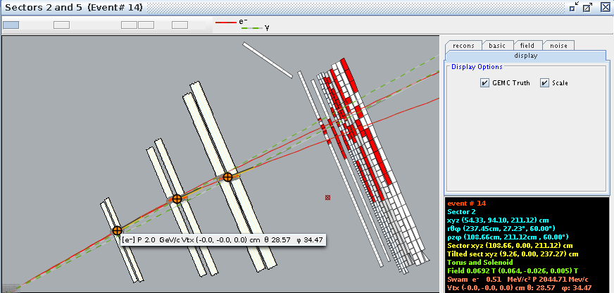
From a GEMC run WITH the Solenoid ced is used to obtain the information from the eg12_rec.ev file.
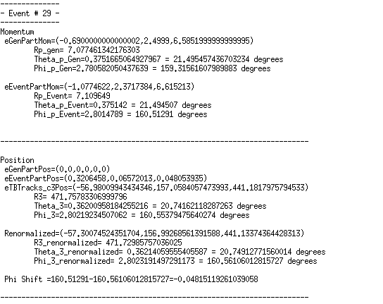
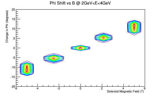
We take the phi angle from the Generated Event momentum as the initial phi angle. The obtain the final phi angle, we can look at the final position of the electron with in the drift chambers.
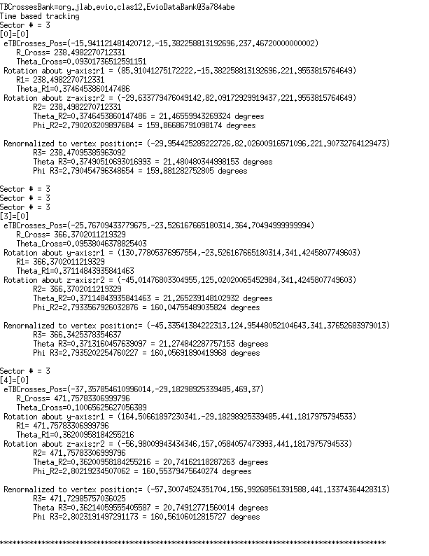
Examining the position from Timer Based Tracking, we can see that after rotations about first the y-axis, then the z-axis transforms from the detector frame of reference to the lab frame of reference.
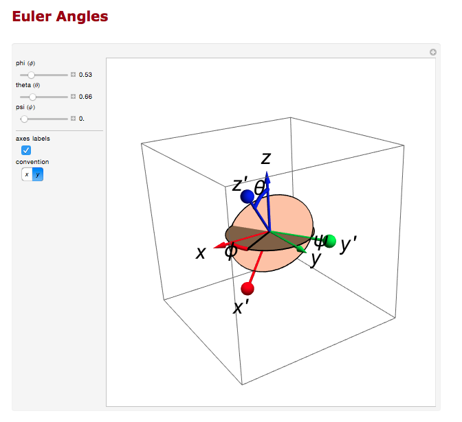
Euler Angles
We can use the Euler angles to perform the rotations.
For the rotation about the y axis.
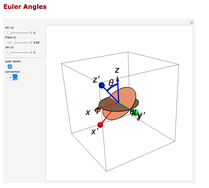
And the rotation about the z axis.
Transformation Matrix
The Euler angles can be applied using a transformation matrix
[math]\left(
\begin{array}{ccc}
\cos (\theta ) & 0 & -\sin (\theta ) \\
0 & 1 & 0 \\
\sin (\theta ) & 0 & \cos (\theta ) \\
\end{array}
\right).\left(
\begin{array}{c}
x \\
y \\
z \\
\end{array}
\right)[/math]
[math]=\left(
\begin{array}{c}
x \cos (\theta )-z \sin (\theta ) \\
y \\
z \cos (\theta )+x \sin (\theta ) \\
\end{array}
\right)[/math]
For event #29, in sector 3, the location of the first interaction is given by
Converting -25 degrees to radians,
[math]\theta =-0.436332[/math]
which is the rotation the detectors are rotated from the y axis.
[math]\left(
\begin{array}{ccc}
\cos (\theta ) & 0 & -\sin (\theta ) \\
0 & 1 & 0 \\
\sin (\theta ) & 0 & \cos (\theta ) \\
\end{array}
\right).\left(
\begin{array}{c}
-15.76 \\
0 \\
237.43 \\
\end{array}
\right)[/math]
[math]=\left(
\begin{array}{c}
86.0588 \\
0. \\
221.845 \\
\end{array}
\right)[/math]
Finding [math]\phi =\frac{120\ 2 \pi }{360};[/math] since "sector -1" =3-1=2*60=120 degrees
[math]\left(
\begin{array}{ccc}
\cos (\phi ) & -\sin (\phi ) & 0 \\
\sin (\phi ) & \cos (\phi ) & 0 \\
0 & 0 & 1 \\
\end{array}
\right).\left(
\begin{array}{c}
86.0588 \\
0. \\
221.845 \\
\end{array}
\right)[/math]
[math]\left(
\begin{array}{c}
-43.0294 \\
74.5291 \\
221.845 \\
\end{array}
\right)[/math]
This shows how the coordinates are transformed and explains the validity of using the TBTracking information to obtain a phi angle in the lab frame.
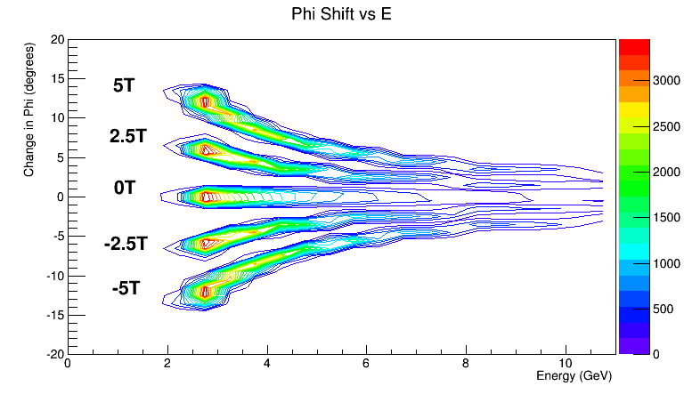
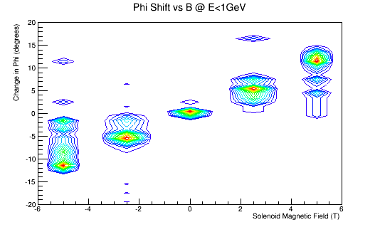
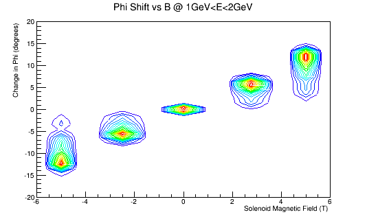
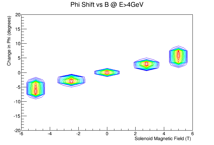
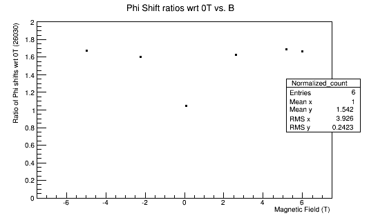
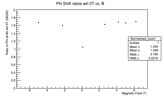
Phi shifts
Cross-section Area
Moller electron Lab Frame
Finding the correct kinematic values starting from knowing the momentum of the Moller (m) electron in the Lab frame,
Using [math]\theta=\arccos(\frac{P_{z(m) Lab}}{P_{(m)Lab}})[/math]
| [math]\Longrightarrow {P_{z(m) Lab}=P_{(m)Lab}\cos(\theta)}[/math]
|
Similarly, [math]\phi=\arccos(\frac{P_{x(m) Lab}}{P_{xy(m) Lab}})[/math]
where [math]P_{xy(m) Lab}=\sqrt{P_{x(m) Lab}^2+P_{y(m)Lab}^2}[/math]
[math]P_{xy(m) Lab}=(P_{x(m) Lab}^2+P_{y(m) Lab}^2)^2[/math]
and using [math]P_{(m)Lab}^2=P_{x(m) Lab}^2+P_{y(m) Lab}^2+P_{z(m) Lab}^2[/math]
this gives [math]P_{(m)Lab}^2=P_{xy(m) Lab}^2+P_{z(m) Lab}^2[/math]
[math]\Longrightarrow P_{(m)Lab}^2-P_{z(m) Lab}^2=P_{xy(m) Lab}^2[/math]
[math]\Longrightarrow P_{xy(m) Lab}=\sqrt{P_{(m)Lab}^2-P_{z(m) Lab}^2}[/math]
which gives[math]\phi = \arccos(\frac{P_{x(m) Lab}}{\sqrt{P_{(m)Lab}^2-P_{z(m) Lab}^2}})[/math]
| [math]\Longrightarrow P_{x(m) Lab}=\sqrt{P_{(m)Lab}^2-P_{z(m) Lab}^2} \cos(\phi)[/math]
|
Similarly, using [math]P_{(m)Lab}^2=P_{x(m) Lab}^2+P_{y(m) Lab}^2+P_{z(m) Lab}^2[/math]
[math]\Longrightarrow P_{(m)Lab}^2-P_{x(m) Lab}^2-P_{z(m) Lab}^2=P_{y(m) Lab}^2[/math]
| [math]P_{y(m) Lab}=\sqrt{P_{(m)Lab}^2-P_{x(m) Lab}^2-P_{z(m) Lab}^2}[/math]
|
Relativistically, the x and y components remain the same in the conversion from the Lab frame to the Center of Mass frame, since the direction of motion is only in the z direction.
| [math]P_{x(m) CM}\Leftrightarrow P_{x(m) Lab}[/math]
|
| [math]P_{y(m) CM}\Leftrightarrow P_{y(m) Lab}[/math]
|
| [math]P_{z(m) CM}=\sqrt{P_{(m)CM}^2-P_{x(m) CM}^2-P_{y(m) CM}^2}[/math]
|
Center of Mass Energy
Using the definition
[math]E^2\equiv p^2c^2+m^2c^4[/math]
[math]\Longrightarrow p^2=\frac {E^2}{c^2}-m^2 c^2[/math]
We can use 4-momenta vectors, i.e. [math]\vec{\mathbf P}\equiv \left(\begin{matrix} E/c\\ p_x \\ p_y \\ p_z \end{matrix} \right)[/math]
we can use the fact that the scalar product of a 4-momenta with itself,
[math]\vec{\mathbf P_1}\cdot \vec{\mathbf P_1}=E_1E_1-\vec p_1\cdot \vec p_1 c^2=m^2c^4=s[/math]
is invariant
Using this, the sum of two 4-momenta forms a 4-vector as well
[math]\vec{\mathbf P_1}+ \vec{\mathbf P_2}= \left( \begin{matrix}E_1+E_2\\\vec p_1 c+\vec p_2 c\end{matrix} \right)=\vec {\mathbf P}[/math]
The length of this four-vector is an invariant as well
[math]\vec{\mathbf P^2}=(\vec{\mathbf P_1}+\vec{\mathbf P_2})^2=(E_1+E_2)^2-(\vec p_1 c+\vec p_2 c)^2=s[/math]
[math]\vec{\mathbf P^2}=(\vec{\mathbf P_1}+\vec{\mathbf P_2})^2=(E_1+E_2)^2-(\vec p_1 +\vec p_2 )^2=s[/math]
(with c=1)
For incoming electrons moving only in the z-direction, we can write
[math]\vec{\mathbf P_1}+ \vec{\mathbf P_2}= \left( \begin{matrix}E_1+E_2\\ 0 \\ 0 \\ p_{1z}+p_{2z}\end{matrix} \right)=\vec{\mathbf P}[/math]
We can perform a Lorentz transformation to the Center of Mass frame, with zero total momentum
[math]\left( \begin{matrix}E_{1 CM}+E_{2 CM}\\ 0 \\ 0 \\ 0\end{matrix} \right)=\left(\begin{matrix}\gamma & 0 & 0 & -\beta \gamma\\0 & 1 & 0 & 0 \\ 0 & 0 & 1 &0 \\ -\beta \gamma & 0 & 0 & \gamma \end{matrix} \right) . \left( \begin{matrix}E_{1 Lab}+E_{2 Lab}\\ 0 \\ 0 \\ p_{1z Lab}+p_{2z Lab}\end{matrix} \right)[/math]
Without knowing the values for gamma or beta, we can use the fact that lengths of the two 4-momenta are invariant
[math]s=\vec{\mathbf P}_{CM}^2=(E_{1 CM}+E_{2 CM})^2-(\vec p_{1 CM}+\vec p_{2 CM})^2[/math]
[math]s=\vec{\mathbf P}_{Lab}^2=(E_{1 Lab}+E_{2 Lab})^2-(\vec p_{1 Lab}+\vec p_{2 Lab})^2[/math]
Setting these equal to each other, we can use this for the collision of two particles of mass m1 and m2. Since the total momentum is zero in the Center of Mass frame, we can express total energy in the center of mass frame as
[math](E_{1 Lab}+E_{2 Lab})^2-(\vec p_{1 Lab}+\vec p_{2 Lab})^2=E_{CM}^2=(E_{1 Lab}+E_{2 Lab})^2-(\vec{p_{1 Lab}}+\vec p_{2 Lab})^2[/math]
[math]E_{CM}=[(E_{1 Lab}+E_{2 Lab})^2-(\vec{p_{1 Lab}}+\vec p_{2 Lab})^2]^{1/2}[/math]
[math]E_{CM}=[E_{1 Lab}^2+2E_{1 Lab}E_{2 Lab}+E_{2 Lab}^2-\vec p_{1 Lab} . \vec p_{2 Lab} -\vec p_{1 Lab} . \vec p_{1 Lab} -\vec p_{2 Lab} . \vec p_{1 Lab} -\vec p_{2 Lab} . \vec p_{2 Lab} ]^{1/2}[/math]
[math]E_{CM}=[(E_{1 Lab}^2- p_{1 Lab}^2 )+(E_{2 Lab}^2-p_{2 Lab}^2 )+2E_{1 Lab}E_{2 Lab}-\vec p_{1 Lab} . \vec p_{2 Lab} -\vec p_{2 Lab} . \vec p_{1 Lab} ]^{1/2}[/math]
[math]E_{CM}=[(E_{1 Lab}^2- p_{1 Lab}^2 )+(E_{2 Lab}^2-p_{2 Lab}^2 )+2E_{1 Lab}E_{2 Lab}-p_{1 Lab} p_{2 Lab}\cos(\theta) - p_{2 Lab} p_{1 Lab}\cos(\theta) ]^{1/2}[/math]
[math]E_{cm}=[m_1^2+m_2^2+2E_{1 Lab}E_{2 Lab}-p_{1 Lab} p_{2 Lab}\cos(\theta) - p_{2 Lab} p_{1 Lab}\cos(\theta) ]^{1/2}[/math]
[math]E_{cm}=[m_1^2+m_2^2+2E_{1 Lab}E_{2 Lab}-2p_{1 Lab} p_{2 Lab}\cos(\theta) ]^{1/2}[/math]
[math]E_{cm}=[m_1^2+m_2^2+2E_{1 Lab}E_{2 Lab}-2p_{1 Lab} p_{2 Lab}\cos(\theta) ]^{1/2}[/math]
Using the relations [math]\beta\equiv \vec p/E\Longrightarrow \vec p=\beta E[/math]
[math]E_{CM}=[m_1^2+m_2^2+2E_1E_2(1-\beta_1\beta_2\cos(\theta))]^{1/2}[/math]
where θ is the angle between the particles.
[math]E_{CM}=[m_1^2+m_2^2+2E_{1 Lab}E_{2 Lab}(1-\beta_1\beta_2\cos(\theta))]^{1/2}[/math]
In the frame where one particle (m2) is at rest
[math]\Longrightarrow \beta_2=0[/math]
[math]\Longrightarrow p_{2 Lab}=0[/math]
which implies,
[math] E_2=[p_{2 Lab}^2+m^2]^{1/2}=m_2[/math]
| [math]E_{cm}=(m_1^2+m_2^2+2E_{1 Lab} m_2)^{1/2}=(.511MeV^2+.511MeV^2+2(\sqrt{(11000 MeV)^2+(.511 MeV)^2})(.511 MeV))^{1/2}\approx 106.031 MeV[/math]
|
where [math]E_{1 Lab}=\sqrt{p_{1 Lab}^2+m_1^2}[/math] in MeV
Inspecting the Lorentz transformation to the Center of Mass frame:
[math]\left( \begin{matrix}E_{1 CM}+E_{2 CM}\\ 0 \\ 0 \\ 0\end{matrix} \right)=\left(\begin{matrix}\gamma & 0 & 0 & -\beta \gamma\\0 & 1 & 0 & 0 \\ 0 & 0 & 1 &0 \\ -\beta \gamma & 0 & 0 & \gamma \end{matrix} \right) . \left( \begin{matrix}E_{1 Lab}+E_{2 Lab}\\ 0 \\ 0 \\ p_{1z Lab}+p_{2z Lab}\end{matrix} \right)[/math]
For the case of a stationary electron, this simplifies to:
[math]\left( \begin{matrix} E_{CM} \\ p_{xCM} \\ p_{y CM} \\ p_{z CM}\end{matrix} \right)=\left(\begin{matrix}\gamma & 0 & 0 & -\beta \gamma\\0 & 1 & 0 & 0 \\ 0 & 0 & 1 &0 \\ -\beta \gamma & 0 & 0 & \gamma \end{matrix} \right) . \left( \begin{matrix}E_{1 Lab}+m\\ 0 \\ 0 \\ p_{1z Lab}+0\end{matrix} \right)[/math]
which gives,
[math]\Longrightarrow\begin{cases}
E_{CM}=\gamma (E_{1 Lab}+m_2)-\beta \gamma p_{1z Lab} \\
p_{zCM}=-\beta \gamma(E_{1 Lab}+m_2)+\gamma p_{1z Lab}
\end{cases}[/math]
Solving for [math]\beta[/math], with [math]p_{zCM}=0[/math]
[math]\Longrightarrow \beta \gamma(E_{1 Lab}+m_2)=\gamma p_{1z Lab}[/math]
| [math]\Longrightarrow \beta=\frac{p_{1 Lab}}{(E_{1 Lab}+m_2)}[/math]
|
Similarly, solving for [math]\gamma[/math] by substituting in [math]\beta[/math]
[math]E_{CM}=\gamma (E_{1 Lab}+m_2)-\frac{p_{1 Lab}}{(E_{1 Lab}+m_2)} \gamma p_{1z Lab}[/math]
[math]E_{CM}=\gamma \frac{(E_{1 Lab}+m_2)^2}{(E_{1 Lab}+m_2)}-\gamma\frac{(p_{1z Lab})^2}{(E_{1 Lab}+m_2)}[/math]
Using the fact that [math]E_{CM}=[(E_{1 Lab}+E_{2 Lab})^2-(\vec p_{1 Lab}+\vec p_{2 Lab})^2]^{1/2}[/math]
[math]E_{CM}=\gamma \frac{E_{CM}^2}{(E_{1 Lab}+m_2)}[/math]
| [math]\Longrightarrow \gamma=\frac{(E_{1 Lab}+m_2)}{E_{CM}}[/math]
|
This gives the momenta of the particles in the center of mass to have equal magnitude, but opposite directions
Using the relation
[math]E_{CM}^2= p_{CM}^2+M^2[/math]
where M is the total mass [math]m_1+m_2[/math]
[math]\Longrightarrow p_{CM}=\sqrt{E_{CM}^2-M^2}[/math]
[math]\Longrightarrow p_{CM}=\sqrt{(106.031 MeV)^2-(2*.511 MeV)^2}\approx 106.026 MeV[/math]
Using the fact that [math]\vec p_{CM}=\vec p_{1 CM}+\vec p_{2 CM}[/math]
| [math] p_{1 CM}=-p_{2 CM}\approx 53.013 MeV[/math]
|
DV_RunGroupC_Moller#Moller_Track_Reconstruction


