Calculating kinematic variables in Moller Lab Frame
Vector Magnitude
The pythagorean theorem is used to take the 3 cartesean components in the Lab frame to find the magnitude of the Moller momentum vector, [math]|\vec{p}_2\ '|[/math].
[math]|\vec{p}_2\ '|=\sqrt{p_x^2+p_y^2+p_z^2}[/math]
Finding the correct kinematic values starting from knowing the momentum of the Moller electron, [math]p^'_{2}[/math] , in the Lab frame,
xz Plane
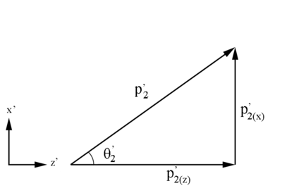 Figure 1: Definition of Moller electron variables in the Lab Frame in the x-z plane.
Using [math]\theta '_2=\arccos \left(\frac{p^'_{2(z)}}{p^'_{2}}\right)[/math]
| [math]\Longrightarrow {p^'_{2(z)}=p^'_{2}\cos(\theta '_2)}[/math]
|
Checking on the sign resulting from the cosine function, we are limited to:
| [math]0^\circ \le \theta '_2 \le 60^\circ \equiv 0 \le \theta '_2 \le 1.046\ Radians[/math]
|
Since,
[math]\frac{p^'_{2(z)}}{p^'_{2}}=cos(\theta '_2)[/math]
[math]\Longrightarrow p^'_{2(z)}\ should\ always\ be\ positive[/math]
xy Plane
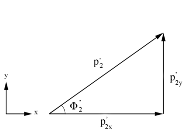 Figure 2: Definition of Moller electron variables in the Lab Frame in the x-y plane.
Similarly, [math]\phi '_2=\arccos \left( \frac{p^'_{2(x) Lab}}{p^'_{2(xy)}} \right)[/math]
where [math]p_{2(xy)}^'=\sqrt{(p_{2(x)}^')^2+(p^'_{2(y)})^2}[/math]
[math](p^'_{2(xy)})^2=(p^'_{2(x)})^2+(p^'_{2(y)})^2[/math]
and using [math]p^2=p_{(x)}^2+p_{(y)}^2+p_{(z)}^2[/math]
this gives [math](p^'_{2})^2=(p^'_{2(xy)})^2+(p^'_{2(z)})^2[/math]
[math]\Longrightarrow (p'_{2})^2-(p'_{2(z)})^2 = (p'_{2(xy)})^2[/math]
[math]\Longrightarrow p_{2(xy)}^'=\sqrt{(p^'_{2})^2-(p^'_{2(z)})^2}[/math]
which gives[math]\phi '_2 = \arccos \left( \frac{p_{2(x)}'}{\sqrt{p_{2}^{'\ 2}-p_{2(z)}^{'\ 2}}}\right)[/math]
| [math]\Longrightarrow p_{2(x)}'=\sqrt{p_{2}^{'\ 2}-p_{2(z)}^{'\ 2}} \cos(\phi)[/math]
|
Similarly, using [math]p_{2}^2=p_{2(x)}^2+p_{2(y)}^2+p_{2(z)}^2[/math]
[math]\Longrightarrow p_{2}^{'\ 2}-p_{2(x)}^{'\ 2}-p_{2(z)}^{'\ 2}=p_{2(y)}^{'\ 2}[/math]
| [math]p_{2(y)}'=\sqrt{p_{2}^{'\ 2}-p_{2(x)}^{'\ 2}-p_{2(z)}^{'\ 2}}[/math]
|
[math]p_{x}[/math] and [math]p_{y}[/math] results based on [math]\phi[/math]
Checking on the sign from the cosine results for [math]\phi '_2[/math]
We have the limiting range that [math]\phi[/math] must fall within:
| [math]-\pi \le \phi '_2 \le \pi\ Radians[/math]
|
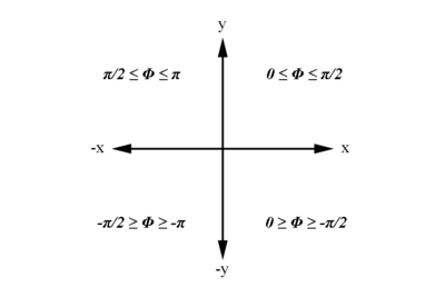
Examining the signs of the components which make up the angle [math]\phi[/math] in the 4 quadrants which make up the xy plane:
| [math]For\ 0 \ge \phi '_2 \ge \frac{-\pi}{2}\ Radians[/math]
|
| px=POSITIVE
|
| py=NEGATIVE
|
| [math]For\ 0 \le \phi '_2 \le \frac{\pi}{2}\ Radians[/math]
|
| px=POSITIVE
|
| py=POSITIVE
|
| [math]For\ \frac{-\pi}{2} \ge \phi '_2 \ge -\pi\ Radians[/math]
|
| px=NEGATIVE
|
| py=NEGATIVE
|
| [math]For\ \frac{\pi}{2} \le \phi '_2 \le \pi\ Radians[/math]
|
| px=NEGATIVE
|
| py=POSITIVE
|
Analysis.groovy
Generating 4-Vector
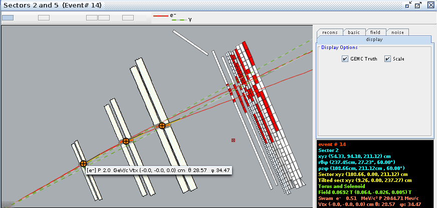
From a GEMC run of solenoid field strength of 0T, the eg12_rec.0.evio output file of the reconstruction is analyzed. The different kinematic variables are displayed as shown:
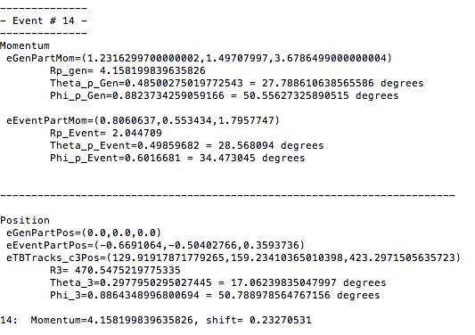
Using the phythagorean theorm to construct the Generated Event momentum vector length, we find:
[math]|\vec{p}_2\ '|=\sqrt{1.23162997^2+1.49707997^2+3.6786499^2}=4.15819983964\ GeV/c[/math]
Using the expression found above for [math]\theta[/math]
[math]\theta '_2=\arccos \left(\frac{p^'_{2(z)}}{p^'_{2}}\right)=\arccos \left(\frac{3.6786499}{4.15819983964}\right)=.4850027502\ Radians=27.7886106387\ degrees[/math]
Similarly, using the expression found for [math]\phi[/math]
[math]\phi '_2=\arccos \left( \frac{p^'_{2(x) Lab}}{p^'_{2(xy)}} \right)=\arccos \left( \frac{1.23162997}{1.93859764252} \right)=.882373425906\ Radians=50.5562732589\ degrees[/math]
where [math]p_{2(xy)}^'=\sqrt{(p_{2(x)}^')^2+(p^'_{2(y)})^2}=\sqrt{1.23162997^2+1.49707997^2}=1.93859764252\ GeV/c[/math]
We take the phi angle from the Generated Event momentum as the initial phi angle.
Change of Generating Vector in eg12 detector
The obtain the final phi angle, we can look at the final position of the electron with in the drift chambers.
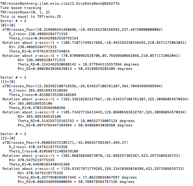
Examining the position from Timer Based Tracking, we can see that after rotations about first the y-axis, then the z-axis transforms from the detector frame of reference to the lab frame of reference.
Transformation Matrix
The Euler angles can be applied using a transformation matrix
[math]\left(
\begin{array}{ccc}
\cos (\theta ) & 0 & -\sin (\theta ) \\
0 & 1 & 0 \\
\sin (\theta ) & 0 & \cos (\theta ) \\
\end{array}
\right).\left(
\begin{array}{c}
x \\
y \\
z \\
\end{array}
\right)[/math][math]=\left(
\begin{array}{c}
x \cos (\theta )-z \sin (\theta ) \\
y \\
z \cos (\theta )+x \sin (\theta ) \\
\end{array}
\right)[/math]
For event #29, in sector 3, the location of the first interaction is given by
Converting -25 degrees to radians,
[math]\theta =-0.436332[/math]
which is the rotation the detectors are rotated from the y axis.
[math]\left(
\begin{array}{ccc}
\cos (\theta ) & 0 & -\sin (\theta ) \\
0 & 1 & 0 \\
\sin (\theta ) & 0 & \cos (\theta ) \\
\end{array}
\right).\left(
\begin{array}{c}
-15.76 \\
0 \\
237.43 \\
\end{array}
\right)[/math][math]=\left(
\begin{array}{c}
86.0588 \\
0. \\
221.845 \\
\end{array}
\right)[/math]
Finding [math]\phi =\frac{120\ 2 \pi }{360};[/math] since "sector -1" =3-1=2*60=120 degrees
[math]\left(
\begin{array}{ccc}
\cos (\phi ) & -\sin (\phi ) & 0 \\
\sin (\phi ) & \cos (\phi ) & 0 \\
0 & 0 & 1 \\
\end{array}
\right).\left(
\begin{array}{c}
86.0588 \\
0. \\
221.845 \\
\end{array}
\right)[/math][math]=\left(
\begin{array}{c}
-43.0294 \\
74.5291 \\
221.845 \\
\end{array}
\right)[/math]
This shows how the coordinates are transformed and explains the validity of using the TBTracking information to obtain a phi angle in the lab frame.


