Using the equation from [1]
[math]\frac{d\sigma}{d\Omega}=\frac{ e^4 }{8E^2}\left \{\frac{1+cos^4\frac{\theta}{2}}{sin^4\frac{\theta}{2}}+\frac{1+sin^4\frac{\theta}{2}}{cos^4\frac{\theta}{2}}+\frac{2}{sin^2\frac{\theta}{2}cos^2\frac{\theta}{2}} \right \}[/math]
where [math]\alpha=\frac{e^2}{\hbar c}\quad with\quad \hbar = c =1[/math]
This can be simplified to the form
[math]\frac{d\sigma}{d\Omega}=\frac{ \alpha^2 }{4E^2}\frac{ (3+cos^2\theta)^2}{sin^4\theta}[/math]
Plugging in the values expected for a scattering electron:
[math]\alpha ^2=5.3279\times 10^{-5}[/math]
[math]E\approx 53 MeV[/math]
Using unit analysis on the term outside the parantheses, we find that the differential cross section for an electron at this momentum should be around
[math]\frac{5.3279\times 10^{-5}}{4\times 2.81\times 10^{15}eV^2}=4.74\times 10^{-21} eV^{-2}=\frac{4.74\times 10^{-21}}{1eV^2}\times \frac{1\times 10^{18}eV^2 }{1\ GeV^2}=\frac{.0047}{GeV^2}[/math]
Using the conversion of
[math]\frac{1}{1GeV^2}=.3894 mb[/math]
[math]\frac{1\ GeV^{-2}}{.3894\ mb}=\frac{.0047\ GeV^{-2}}{x\ mb}[/math]
The trigonometric function part of the equation comes out to it's minimum of 9 at 90 degrees.
[math]\frac{(3+Cos^2(90))^2}{Sin^4(90)}=9[/math]
We find that the differential cross section scale is [math]\frac{d\sigma}{d\Omega}\approx 1.8\times 10^{-3}mb \times 9=16.2\mu b[/math]
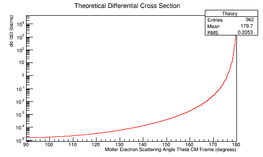
Figure 5a: The theoretical Moller electron differential cross-section for an incident 11 GeV(Lab) electron in the Center of Mass frame of reference.
Converting the number of electrons scattered per angle theta to barns, we can use the relation
[math]L=\frac{i_{scattered}}{\sigma} \approx i_{scattered}\times \rho_{target}\times l_{target}[/math]
where ρtarget is the density of the target material, ltarget is the length of the target, and iscattered is the number of incident particles scattered.
This gives, for LH2:
[math]\rho_{target}\times l_{target}=\frac{70.85 kg}{1 m^3}\times \frac{1 mole}{2.02 g} \times \frac{1000g}{1 kg} \times \frac{6\times10^{23} atoms}{1 mole} \times \frac{1m^3}{(100 cm)^3} \times \frac{1 cm}{ } \times \frac{10^{-24} cm^{2}}{barn} =2.10\times 10^{-2} barns[/math]
Using the number of incident electrons,
[math]\frac{1}{\rho_{target}\times l_{target} \times 4\times 10^7}=1.19\times 10^{-6} barns[/math]
We can use this number to scale the number of electrons per angle to a differential cross-section in barns. Using the plot of the Moller electron scattering angle theta in the Center of Mass frame,
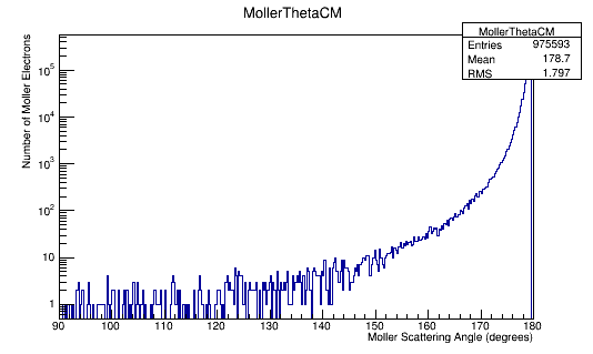
Figure 5b: The Moller electron scattering angle theta distribution for an incident 11 GeV(Lab) electron in the Center of Mass frame of reference.
We can rescale and combine the theoretical differential cross-section for one electron.
TH1F *Combo=new TH1F("TheoryExperiment","Theoretical and Experimental Differential Cross-Section CM Frame",360,90,180);
Combo->Add(MollerThetaCM,1.19e-6);
Combo->Draw();
Theory->Draw("same");

