Calculating the differential cross-sections for the different materials, and placing them as well as the theoretical differential cross-section into a plot:

Comparing this to the theoretical differential cross section

As shown above , we find that the differential cross section scale is [math]\frac{d\sigma}{d\Omega}\approx 16.2\times 10^{-2}mb=16.2\mu b[/math]

Converting the number of electrons to barns,

[math]L=\frac{i_{scattered}}{\sigma} \approx i_{scattered}\times \rho_{target}\times l_{target}[/math]

where ρ_target is the density of the target material, l_target is the length of the target, and i_scattered is the number of incident particles scattered.

For LH2:

[math]\rho_{target}\times l_{target}=\frac{70.85 kg}{1 m^3}\times \frac{1 mole}{2.02 g} \times \frac{1000g}{1 kg} \times \frac{6\times10^{23} atoms}{1 mole} \times \frac{1m^3}{(100 cm)^3} \times \frac{1 cm}{ } \times \frac{10^{-24} cm^{2}}{barn} =2.10\times 10^{-2} barns[/math]

[math]\frac{1}{\rho_{target}\times l_{target} \times 4\times 10^7}=1.19\times 10^{-6} barns[/math]

For Carbon:

[math]\rho_{target}\times l_{target}=\frac{2.26 g}{1 cm^3}\times \frac{1 mole}{12.0107 g} \times \times \frac{6\times10^{23} atoms}{1 mole} \times \frac{1 cm}{ } \times \frac{10^{-24} cm^{2}}{barn} =1.13\times 10^{-1} barns[/math]

[math]\frac{1}{\rho_{target}\times l_{target} \times 4\times 10^7}=2.21\times 10^{-7} barns[/math]

For Ammonia:

[math]\rho_{target}\times l_{target}=\frac{.8 g}{1 cm^3}\times \frac{1 mole}{17 g} \times \frac{6\times10^{23} atoms}{1 mole} \times \frac{1 cm}{ } \times \frac{10^{-24} cm^2}{barn} =2.82\times 10^{-2} barns[/math]

[math]\frac{1}{\rho_{target}\times l_{target} \times 4\times 10^7}=8.87\times 10^{-7} barns[/math]

Combing plots in Root:

new TBrowser();
TH1F *LH2=new TH1F("LH2","LH2",360,90,180);
LH2->Add(MollerThetaCM,1.19e-6);
LH2->Draw();

TH1F *C12=new TH1F("C12","C12",360,90,180);
C12->Add(MollerThetaCM,2.21e-7);
C12->Draw();

TH1F *NH3=new TH1F("NH3","NH3",360,90,180);
NH3->Add(MollerThetaCM,8.87e-7);
NH3->Draw();
LH2->Draw("same");
C12->Draw("same");
Theory->Draw("same");

Molar Mass of Target Material

Material	Molar Mass (g/mole)
NH3	17
C	12
LH2	2

Number of Electrons in Target Material

Material	Number of Electrons
NH3	10
C	6
LH2	2

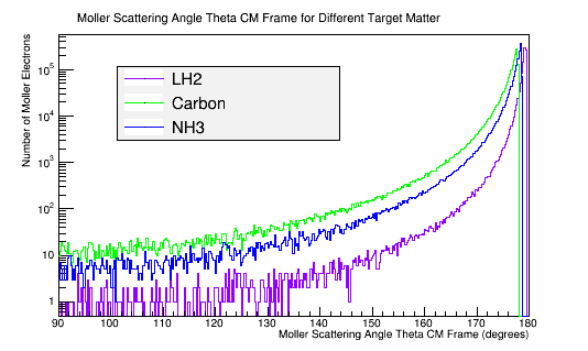
[math]\Longrightarrow[/math]The greater the molar mass, the smaller the solid angle into which the Moller electron will scatter.

Comparing this with a plot of the Moller scattering angle theta,

Figure 8d: The Moller scattering angle theta for 4E7 incident 11 GeV electrons in the Center of Mass frame of reference for 3 different target materials.

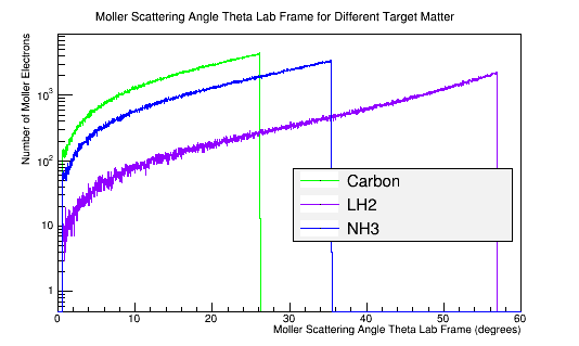
Density of target material

C=2.26 g/cm³

NH3=.86g/cm³

LH2=.07g/cm³

[math]\Longrightarrow[/math]The greater the density, the smaller the solid angle into which the Moller electron will scatter.

Figure 8b: The Moller electron momentum distribution for 4E7 incident 11 GeV electrons in the Lab frame of reference.

---

Links

Back