Difference between revisions of "A W thesis old"
| Line 1: | Line 1: | ||
| + | =Results and Conclusion= | ||
| + | This thesis set out to measure the detection limit improvement of coincidence photon activation analysis over the more common photon activation analysis method. By requiring detected photons to be in coincidence, it is thought that the detection limit can be improved over standard PAA. The following sections contain the results obtain performing singles and coincidence counting for PAA. | ||
| + | |||
| + | |||
| + | ==Detection Limit of PAA for a Yt-89 foil== | ||
| + | |||
| + | |||
| + | |||
| + | The detection limit represents a quantitative measurement of the lowest number of nuclei that may be observed. This quantity may be expressed in units of parts-per-million (PPM) or in the equivalent units of (<math>\mu g/g</math>). | ||
| + | |||
| + | The concept of photon activation analysis relies on activating a nucleus by using a high energy photon to eject one or more nucleons (protons or neutrons). The nuclei that have had one or more nucleons removed are typically unstable and decay. One can determine this rate of decay in terms of the probability of decay , <math>\lambda.</math>. If I let N(t) represent the number of radioactive nuclei at time t I can estimate the change in this number by | ||
| + | |||
| + | ===Radioactive decay=== | ||
| + | |||
| + | :<math>N(t) -N(t + \Delta t) = N(t) (\lambda \Delta t)</math> | ||
| + | |||
| + | dividing by <math>\Delta t</math> and taking the limit of <math>\Delta t \rightarrow 0</math> | ||
| + | :<math>\Rightarrow \lim_{\Delta t \rightarrow 0} \frac{N(t+\Delta t) - N(t) }{\Delta t} = \frac{dN}{dt} = - \lambda N(t)</math> | ||
| + | |||
| + | The solution to the above differential is | ||
| + | |||
| + | :<math>N(t) = N_0 e^{\lambda t}</math> | ||
| + | |||
| + | If I want to know the time required until the original number of activated nuclei (<math>N_0</math>) has been cut in half | ||
| + | |||
| + | :<math>\Rightarrow \frac{1}{2} = e^{\lambda t_{1/2}} \Rightarrow t_{1/2} = \frac{\ln 2}{\lambda}</math> | ||
| + | |||
| + | The half life of a decaying nucleus is inversely proportional to the probability of decay. | ||
| + | |||
| + | The activity<math> (A)</math> of a sample of radioactive nuclei is defined as the rate of the decay and is given by | ||
| + | |||
| + | :<math>A = \lambda N(t)</math> | ||
| + | |||
| + | The above has the units of decays per sec , or Bacquerel. | ||
| + | |||
| + | The nucleus Y-88 for example has a half life of 106.6 days. If I measure the activity of the sample at time <math>t</math> then the number of radioactive nuclei at time <math>t</math> is given by | ||
| + | |||
| + | |||
| + | : <math>N= A \frac{t_{1/2}}{\ln 2} = \left ( 1.33 \times 10^7 \mbox {s} \right ) A</math> | ||
| + | |||
| + | where <math>A</math> is the number of measured decays per sec. | ||
| + | |||
| + | The isotope Y-88 was produced by ejecting a neutron from the stable Y-89 nucleus using a photon having more energy enough energy to overcome the binding energy. | ||
| + | |||
| + | Neutron Separation Energy=<math>S_n = B({A \atop Z} X_{N})-B({{A-1} \atop Z} X_{N-1})</math> | ||
| + | |||
| + | <math>B({89 \atop39} Y_{50}) = 775538.048 keV</math> | ||
| + | <math>B({88 \atop39} Y_{49}) = 764061.688 keV</math> | ||
| + | :<math>S_n = B({89 \atop 39} X_{50})-B({{88} \atop 39} Y_{49})=775538.048-764061.688=11.47636</math> MeV | ||
| + | A photon needs to have at least 11.5 MeV of energy to eject one neutron from Y-89. | ||
| + | |||
| + | To determine the number of Y-89 atoms that were converted you need to know the efficiency of the detector (<math>\epsilon</math>), the branching ratio of the photons measured (Br), and the probability of creating Y-88 from Y-89. The detector efficiency for measuring a 898 keV photon using an HpGe detector was (0.7830 +/- 0.0471) % and ( 0.3119 +/- 0.0310) % for 1836.1 keV photons. The Y-88 activity was extrapolated to be 300 Hz using the known half life and the observed efficiency corrected count rate in a HpGe detector. The branching ratio for the 898 keV line is almost unity (95 %) indicating that after irradiation there were 300 Y-88 nuclei decaying per second or | ||
| + | :: <math>N= A \frac{t_{1/2}}{\ln 2} = \left ( 1.33 \times 10^7 \mbox {s} \right ) 300 Hz = 4 \times 10^{9}</math> activated Nuclei. | ||
| + | |||
| + | To determine how many Y-89 atoms had a neutron removed we would need to know what fraction of all the photon induced reaction are single neutron knockout. | ||
| + | |||
| + | The number of atoms in a Yt foil having a mass of <math>0.0496 \pm 0.002</math> g is | ||
| + | |||
| + | : <math>n_{Y-89} = (0.0496 \pm 0.002 g) \times \left ( \frac {1 \mbox{mole}}{88.90585 \mbox{g}}\right ) \times \left ( \frac {6 \times 10^{23} \mbox{atoms}}{ \mbox{mole}}\right ) = 3.35 \times 10^{20}</math> atoms | ||
| + | |||
| + | ==Activation efficiency for Y-88== | ||
| + | |||
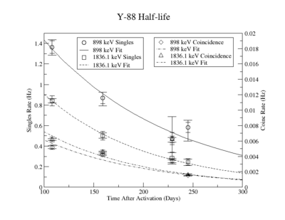
| + | It is well understood that radioactive materials decay as an exponential function of time. We can therefore use the measured signals of the Y-88 sample fitted to an exponential curve to find the initial number of atoms in the foil. The exponential fit was extrapolated back to the initial time t=0 when the foil was activated. We want to convert this initial rate (Hz) into units of Curie. The half-life of Y-88 is well know, 106.63 days, and was used to calculate the decay constant <math>\lambda</math>. Using the relationship between activity and the number density <math>A=\lambda N</math> we can find <math>N_0</math> for t=0. | ||
| + | |||
| + | The yttrium foil's mass was weighted at the IAC and found to be 0.0288 +/- 0.0002 g. Using Avogadro's number, <math>N_a</math>, and the isotopic mass of Y-89, <math>m_i=88.905848 \frac{g}{mol}</math>, we can plug into the following equation: <math>Number of atoms = \frac{mN_a}{m_i}</math>. The foil is predicted to contain <math>1.95\times 10^{20} \pm 1.35\times 10^{18}</math> atoms of Y-89. | ||
| + | |||
| + | Taking to ratio of <math>N_0</math> and the number of atoms will measure the accelerator beam's efficiency at activating the sample. Using the above number of atoms and using the average <math>N_0</math> found previously, we get a ratio of <math> (19.7 \pm 2.72) \times 10^{-12}</math>. | ||
| + | |||
| + | |||
| + | ---------------- | ||
| + | |||
| + | During activation of the Y-90 sample, a neutron can be knocked out of the Y-90 nucleus leaving behind the Y-88 nucleus in an excited state. The Y-88 nucleus has a decay half life of 106.63 days. During the irradiation you have two competing processes, the knocking out of a neutron to make Y-88 and the decay of Y-88 while you are activating it. | ||
| + | |||
| + | ==Determining the lowest measurable activity== | ||
| + | |||
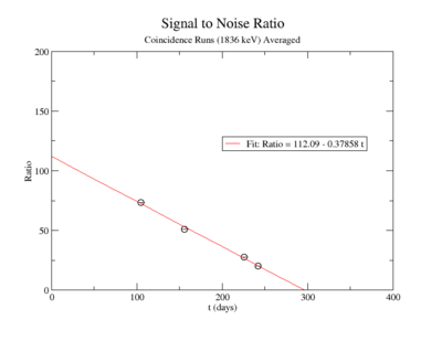
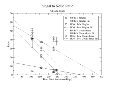
| + | The lowest activity of Y-88 that the apparatus could measure is predicted by extrapolating the measured signal to noise ratio forward in time until it is zero. The signal to noise ratio fits shown in figureXX.YY were used for this extrapolation. Beyond this point in time, we will not be able to distinguish the signal from the background noise and measurements will no longer be possible with this apparatus. This time for the SNR to be zero was used in the exponential decay function <math>N(t)=N_0e^{-\lambda t}</math> to find the lowest measurable activity, <math> N(t_{final}) </math>. This activity is reported in Table XX.III for singles and coincidence measurements of both photon energies. | ||
| + | |||
| + | |||
=Apparatus= | =Apparatus= | ||
Latest revision as of 17:37, 5 May 2015
Results and Conclusion
This thesis set out to measure the detection limit improvement of coincidence photon activation analysis over the more common photon activation analysis method. By requiring detected photons to be in coincidence, it is thought that the detection limit can be improved over standard PAA. The following sections contain the results obtain performing singles and coincidence counting for PAA.
Detection Limit of PAA for a Yt-89 foil
The detection limit represents a quantitative measurement of the lowest number of nuclei that may be observed. This quantity may be expressed in units of parts-per-million (PPM) or in the equivalent units of ().
The concept of photon activation analysis relies on activating a nucleus by using a high energy photon to eject one or more nucleons (protons or neutrons). The nuclei that have had one or more nucleons removed are typically unstable and decay. One can determine this rate of decay in terms of the probability of decay , . If I let N(t) represent the number of radioactive nuclei at time t I can estimate the change in this number by
Radioactive decay
dividing by and taking the limit of
The solution to the above differential is
If I want to know the time required until the original number of activated nuclei () has been cut in half
The half life of a decaying nucleus is inversely proportional to the probability of decay.
The activity of a sample of radioactive nuclei is defined as the rate of the decay and is given by
The above has the units of decays per sec , or Bacquerel.
The nucleus Y-88 for example has a half life of 106.6 days. If I measure the activity of the sample at time then the number of radioactive nuclei at time is given by
where is the number of measured decays per sec.
The isotope Y-88 was produced by ejecting a neutron from the stable Y-89 nucleus using a photon having more energy enough energy to overcome the binding energy.
Neutron Separation Energy=
- MeV
A photon needs to have at least 11.5 MeV of energy to eject one neutron from Y-89.
To determine the number of Y-89 atoms that were converted you need to know the efficiency of the detector (), the branching ratio of the photons measured (Br), and the probability of creating Y-88 from Y-89. The detector efficiency for measuring a 898 keV photon using an HpGe detector was (0.7830 +/- 0.0471) % and ( 0.3119 +/- 0.0310) % for 1836.1 keV photons. The Y-88 activity was extrapolated to be 300 Hz using the known half life and the observed efficiency corrected count rate in a HpGe detector. The branching ratio for the 898 keV line is almost unity (95 %) indicating that after irradiation there were 300 Y-88 nuclei decaying per second or
- activated Nuclei.
To determine how many Y-89 atoms had a neutron removed we would need to know what fraction of all the photon induced reaction are single neutron knockout.
The number of atoms in a Yt foil having a mass of g is
- atoms
Activation efficiency for Y-88
It is well understood that radioactive materials decay as an exponential function of time. We can therefore use the measured signals of the Y-88 sample fitted to an exponential curve to find the initial number of atoms in the foil. The exponential fit was extrapolated back to the initial time t=0 when the foil was activated. We want to convert this initial rate (Hz) into units of Curie. The half-life of Y-88 is well know, 106.63 days, and was used to calculate the decay constant . Using the relationship between activity and the number density we can find for t=0.
The yttrium foil's mass was weighted at the IAC and found to be 0.0288 +/- 0.0002 g. Using Avogadro's number, , and the isotopic mass of Y-89, , we can plug into the following equation: . The foil is predicted to contain atoms of Y-89.
Taking to ratio of and the number of atoms will measure the accelerator beam's efficiency at activating the sample. Using the above number of atoms and using the average found previously, we get a ratio of .
During activation of the Y-90 sample, a neutron can be knocked out of the Y-90 nucleus leaving behind the Y-88 nucleus in an excited state. The Y-88 nucleus has a decay half life of 106.63 days. During the irradiation you have two competing processes, the knocking out of a neutron to make Y-88 and the decay of Y-88 while you are activating it.
Determining the lowest measurable activity
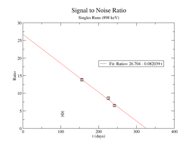
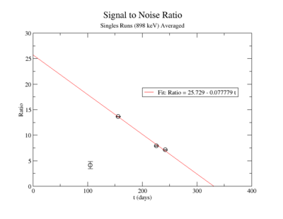
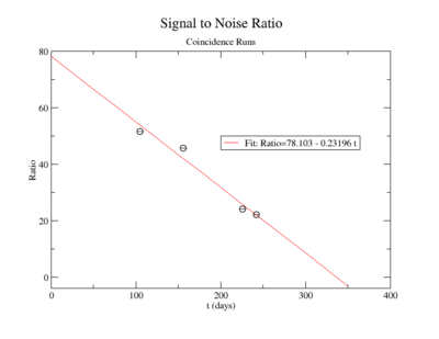
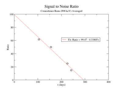
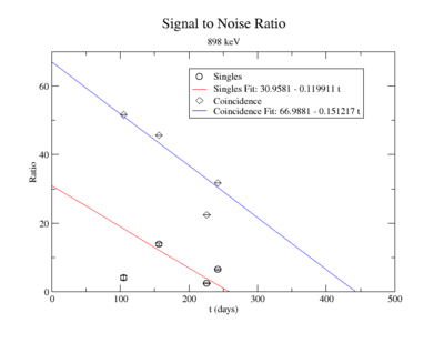
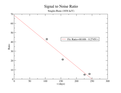
The lowest activity of Y-88 that the apparatus could measure is predicted by extrapolating the measured signal to noise ratio forward in time until it is zero. The signal to noise ratio fits shown in figureXX.YY were used for this extrapolation. Beyond this point in time, we will not be able to distinguish the signal from the background noise and measurements will no longer be possible with this apparatus. This time for the SNR to be zero was used in the exponential decay function to find the lowest measurable activity, . This activity is reported in Table XX.III for singles and coincidence measurements of both photon energies.
Apparatus
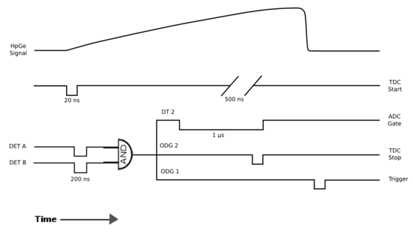
The coincidence counting set-up and modules path are as follows. A source is set atop a base constructed of hydrogen dense blocks. These were chosen to reduce the number of background energy spikes detected. The source is placed an equal distance from decorator A and detector B. Detector A is positioned directly above the source. A high-purity germanium detector is being utilized for this set-up. The one outgoing signal enters a ORTEC 673 Spectroscopy Amplifier and the outgoing signal then passes through a CANBERRA CFD 2035A. The signal can then enter an optional CAEN CFD to produce a time delay, or can pass directly into a channel (1) of the Level Translator. The second outgoing signal from the Spec Amp goes to a peak sensing CAEN V785N. The output from this module goes to the DAQ. Perpendicular from detector A and placed an equal distance from the source is detector B. This detector can either be a NaI-3 or a germanium detector depending on the source being counted. Detector B’s signal goes to a Post Amplifier and one outgoing signal goes to the above mentioned CAEN V785N and also to the DAQ. The second signal enters a CANBERRA CFD 2035A. The outgoing signal goes to a different channel (4) of the same Level Translator. A ribbon cable on the Level Translator module goes to a Time-to-Digital Converter (TDC) CAEN V775 that is operating in common start mode. Both channels (1 and 4) of the Level Translator outgoing signal pass to a 3-fold Logic Unit which is used in both OR mode and AND mode to see coincidence lines. This data is collected in the Trig DAQ.
898 keV signal table
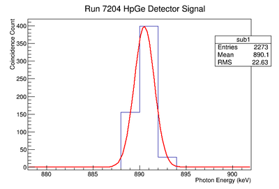
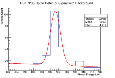
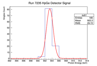
Re-Fit of Run 7203 without Event Cuts
Re-Fit of Run 7203 without Event Cuts and Scaled by 1.66
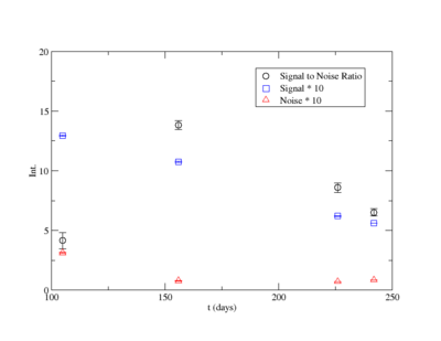
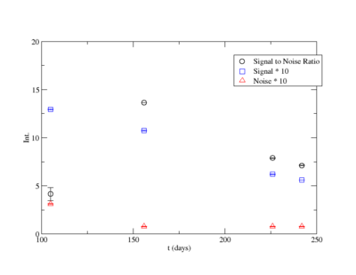
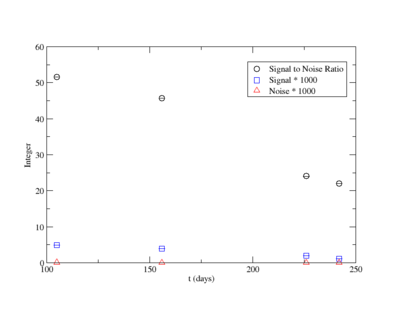
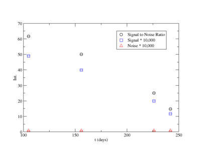
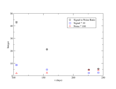
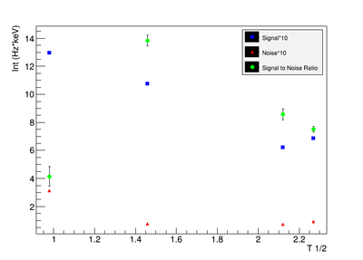
Signal, Noise, and Signal to Noise Ratio plots for 898 keV singles runs.
Averaging over the last three noise values:
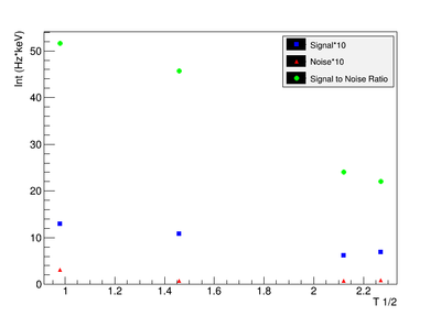
Signal, Noise, and Signal to Noise Ratio plots for 898 keV coincidence runs.
Averaging over the noise values:
Signal to Noise Ratio (Singles and Coincidence):
1836 keV signal table
1836.1 keV Signal Table
Re-Fit of Run 7203 without Event Cuts
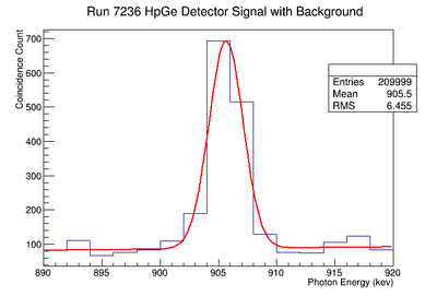
Re-Fit of Run 7236 without Event Cuts
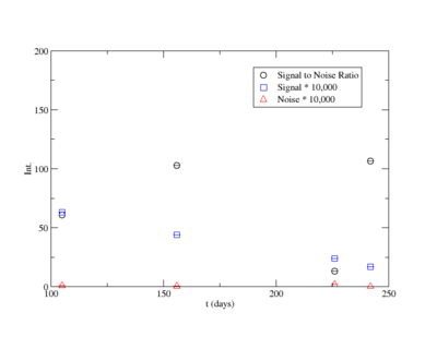
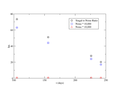
Signal, Noise, and Signal to Noise Ratio plots for 1836 keV singles runs.
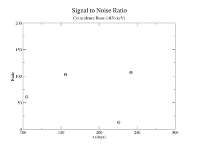
Signal, Noise, and Signal to Noise Ratio plots for 1836 keV coincidence runs.
Averaging over the noise values:
Signal to Noise Ratio (Singles and Coincidence):
Error analysis
Half-life
Values
898 keV Singles
| Days | Trig | Energy Window | Energy Calibration | Linear Fit of Background | Gaussian Integration of Signal | Total Systematic Error | |
| 105 | 0.98 | sing | |||||
| 156 | 1.46 | sing | |||||
| 226 | 2.12 | sing | |||||
| 242 | 2.27 | sing |
898 keV Coincidence
| Days | Trig | Energy Window | Energy Calibration | Linear Fit of Background | Gaussian Integration of Signal | Coincidence Energy | Total Systematic Error | |
| 105 | 0.98 | coin | ||||||
| 156 | 1.46 | coin | ||||||
| 226 | 2.21 | coin | ||||||
| 242 | 2.27 | coin |
1836.1 keV Singles
| Days | Trig | Energy Window | Energy Calibration | Linear Fit of Background | Gaussian Integration of Signal | Total Systematic Error | |
| 105 | 0.98 | sing | |||||
| 156 | 1.46 | sing | |||||
| 226 | 2.12 | sing | |||||
| 242 | 2.27 | sing |
1836.1 keV Coincidence
| Days | Trig | Energy Window | Energy Calibration | Linear Fit of Background | Gaussian Integration of Signal | Coincidence Energy Cut | Total Systematic Error | |
| 105 | 0.98 | coin | ||||||
| 156 | 1.46 | coin | ||||||
| 226 | 2.12 | coin | ||||||
| 242 | 2.27 | coin |
Percent Error
898 keV Singles
| Days | Trig | Energy Window | Energy Calibration | Linear Fit of Background | Gaussian Integration of Signal | Total Systematic Error | |
| 105 | 0.98 | sing | |||||
| 156 | 1.46 | sing | |||||
| 226 | 2.12 | sing | |||||
| 242 | 2.27 | sing |
898 keV Coincidence
| Days | Trig | Energy Window | Energy Calibration | Linear Fit of Background | Gaussian Integration of Signal | Coincidence Energy | Total Systematic Error | |
| 105 | 0.98 | coin | ||||||
| 156 | 1.46 | coin | ||||||
| 226 | 2.21 | coin | ||||||
| 242 | 2.27 | coin |
1836.1 keV Singles
| Days | Trig | Energy Window | Energy Calibration | Linear Fit of Background | Gaussian Integration of Signal | Total Systematic Error | |
| 105 | 0.98 | sing | |||||
| 156 | 1.46 | sing | |||||
| 226 | 2.12 | sing | |||||
| 242 | 2.27 | sing |
1836.1 keV Coincidence
| Days | Trig | Energy Window | Energy Calibration | Linear Fit of Background | Gaussian Integration of Signal | Coincidence Energy Cut | Total Systematic Error | |
| 105 | 0.98 | coin | ||||||
| 156 | 1.46 | coin | ||||||
| 226 | 2.12 | coin | ||||||
| 242 | 2.27 | coin |
SNR
The signal to noise ratio is
| Days | Trig | SNR | Statistical Error | Systematic Error | |
| 105 | 0.98 | sing | 42.07 | ||
| coin | 9.65 | ||||
| 156 | 1.46 | sing | 21.52 | ||
| coin | 7.16 | ||||
| 226 | 2.12 | sing | 4.64 | ||
| coin | 9.65 | ||||
| 242 | 2.27 | sing | 5.43 | ||
| coin | 2.49 |
=other
| Energy | Trig | (days) | (before efficiency) | (after efficiency) | |||
| 898 | sing | 130.39 +/- 26.26 | 1.281e-8 +/- 2.236e-9 | 1.636e-6 +/- 2.957e-7 | 383.63 | 1.351e-7 +/- 7.551e-8 | 0.0826 +/- 0.0485 |
| coin | 108.18 +/- 4.89 | 6.411e-11 +/- 1.314e-12 | 3.794e-8 +/- 2.633e-9 | 483.60 | 1.636e-9 +/- 3.954e-10 | 0.0431 +/- 0.0108 | |
| 1836.1 | sing | 106.16 +/- 8.63 | 9.634e-9 +/- 1.089e-9 | 3.089e-6 +/- 3.619e-7 | 264.94 | 5.519e-7 +/- 8.705e-8 | 0.1787 +/- 0.0351 |
| coin | 100.10 +/- 4.0 | 8.147e-11 +/- 1.670e-12 | 4.171e-8 +/- 1.860e-9 | 305.63 | 5.721e-9 +/- 1.238e-9 | 0.1371 +/- 0.0303 |
898 keV Signal and Background Noise Table
| Run # | Area of Signal | Area of Background | Signal to Noise Ratio |
| 7203 | 130.17 | 120.59 | 1.08 |
| 7204 | 825.34 | 558.66 | 1.48 |
| 7235 | 194.38 | 60.23 | 3.23 |
| 7236 | 1429.75 | 436.93 | 3.27 |
1836.1 keV Signal and Background Noise Table
| Run # | Area of Signal | Area of Background | Signal to Noise Ratio |
| 7203 | 83.29 | 24.73 | 3.37 |
| 7204 | 944.58 | 101.68 | 9.29 |
| 7235 | 82.25 | 20.90 | 3.94 |
| 7236 | 1849.86 | 97.64 | 18.95 |
HpGe Detector
| Run | Source | Energy | Expected rate (Hz) | HpGe Det B Rate (ADC 7) (Hz) | HpGe Eff (%) |
| 7027 | Na-22 | 511 | 1589.218 +/- 49.425 | 18.07 +/- 0.111 | 1.137 +/- 0.0317 |
| 7025 | Cs-137 | 661.657 | 2548.03 +/- 80.008 | 25.468+/- 0.172 | 0.9995 +/- 0.0321 |
| 7029 | Mn-54 | 834.848 | 41.405 +/- 1.300 | 0.485 +/- 0.014 | 1.171 +/- 0.0427 |
| 7026 | Co-60 | 1173.228 | 1876.619 +/- 58.926 | 11.03 +/- 0.106 | 0.588 +/- 0.0328 |
| 7027 | Na-22 | 1274.537 | 888.264 +/- 27.625 | 4.857 +/- 0.034 | 0.5468 +/- 0.0319 |
| 7026 | Co-60 | 1332.492 | 1878.167 +/- 58.974 | 9.584 +/- 0.023 | 0.510 +/- 0.0315 |
Extrapolated Efficiency
| Source | Energy | HpGe Eff (%) |
| Y-88 | 898 | 1.036 +/- 0.0226 |
| Y-88 | 1836.1 | 0.1983 +/- 0.0178 |
Exp Fit including Cs-137
  1  Constant     7.96246e-01   6.78458e-02   6.83891e-05  -2.33206e-03
  2  Slope       -1.07699e-03   7.10063e-05   7.15739e-08  -2.09517e+00
f(x) = exp(p0+p1*x).
Extrapolated Efficiency
| Source | Energy | HpGe Eff (%) |
| Y-88 | 898 | 0.8429 +/- 0.0034 |
| Y-88 | 1836.1 | 0.3069 +/- 0.0192 |
| Energy | Trig | (before efficiency) |
| 898 | sing | 1.281e-8 +/- 2.254e-9 |
| coin | 6.411e-11 +/- 3.572e-12 | |
| 1836.1 | sing | 9.634e-9 +/- 1.102e-9 |
| coin | 8.147e-11 +/- 2.987e-12 |
Exp Fit including all Na-22 points and excluding Mn-54
  1  Constant     6.36491e-01   4.70444e-02   1.00271e-05  -3.28621e-03
  2  Slope       -9.81232e-04   5.68236e-05   1.21109e-08  -1.59453e+00
Extrapolated Efficiency
| Source | Energy | HpGe Eff (%) |
| Y-88 | 898 | 0.7830 +/- 0.0471 |
| Y-88 | 1836.1 | 0.3119 +/- 0.0310 |
| Energy | Trig | (before efficiency) |
| 898 | sing | 1.281e-8 +/- 2.254e-9 |
| coin | 6.411e-11 +/- 3.572e-12 | |
| 1836.1 | sing | 9.634e-9 +/- 1.102e-9 |
| coin | 8.147e-11 +/- 2.987e-12 |
Efficiency on 2/28/2014
| Run | Source | Energy | Expected rate (Hz) | HpGe Det B Rate (ADC 7) (Hz) | HpGe Eff (%) |
| 7028 | Ba-133 | 80.9971 | 1067.468 +/- 1.131 | 14.483 +/- 1.442 | 1.357 |
| 7028 | Ba-133 | 276.3997 | 221.297 +/- 0.2345 | 4.239 +/- 0.9671 | 1.916 |
| 7028 | Ba-133 | 302.8510 | 574.310 +/- 0.6085 | 9.523 +/- 0.5539 | 1.658 |
| 7028 | Ba-133 | 356.0134 | 1941.418 +/- 2.057 | 27.130 +/- 1.316 | 1.397 |
| 7028 | Ba-133 | 383.8480 | 278.416 +/- 0.2950 | 3.982 +/- 0.2440 | 1.430 |
| 7027 | Na-22 | 511 | 1589.218 +/- 1.842 | 17.545 +/- 0.4560 | 1.104 |
| 7025 | Cs-137 | 661.657 | 2548.022 +/- 2.222 | 25.622+/- 0.3286 | 1.006 |
| 7029 | Mn-54 | 834.848 | 4032.782 +/- 0.0114 | 0.2911 +/- 0.1667 | 0.0072 |
| 7026 | Co-60 | 1173.228 | 1876.619 +/- 0.2687 | 11.062 +/- 0.1215 | 0.589 |
| 7027 | Na-22 | 1274.537 | 888.264 +/- 1.029 | 4.685 +/- 0.0825 | 0.527 |
| 7026 | Co-60 | 1332.492 | 1878.167 +/- 0.2690 | 9.616 +/- 0.1181 | 0.512 |
| Run | Source | Energy | Expected rate (Hz) | NaI Det B Rate (ADC 7) (Hz) | NaI Eff (%) |
| 7027 | Na-22 | 511 | 1589.218 +/- 49.425 | 14.86 +/- 0.0945 | 0.9351 +/- 0.0317 |
| 7025 | Cs-137 | 661.657 | 2548.03 +/- 80.008 | 23.45 +/- 0.9729 | 0.9203 +/- 0.0520 |
| 7026 | Co-60 | 1173.228 | 1876.619 +/- 58.926 | 8.001 +/- 0.0953 | 0.4264 +/- 0.0336 |
| 7027 | Na-22 | 1274.537 | 888.264 +/- 27.625 | 4.05 +/- 0.0247 | 0.4559 +/- 0.0317 |
| 7026 | Co-60 | 1332.492 | 1878.167 +/- 58.974 | 7.234 +/- 0.1675 | 0.3852 +/- 0.0390 |
Signal, Noise, and Signal to Noise Ratio plots for 898 keV singles runs.
Signal, Noise, and Signal to Noise Ratio plots for 898 keV coincidence runs.
| Trig | Fit Parameters | Signal Area | Noise Area | SNR | |||||
| 0.98 | sing | 897.260 +/- 0.0047 | 0.7074 +/- 0.0280 | A=0.725 +/- 0.0129 | B= 8.448e-4+/- 4.457e-5 | C=-0.7355 +/- 0.0408 | 0.9938 +/- 0.0054 | 0.3039 +/- 0.0380 | 3.270 +/- 0.0243 |
| coin | +/- | +/- | A= +/- | B= +/- | C= +/- | +/- | +/- | +/- | |
| 2.27 | sing | 903.482 +/- 0.0064 | 0.6595 +/- 0.0877 | A= 0.3199 +/- 0.0156 | B= -7.248e-4+/- 9.968e-7 | C= 6.816e-1 +/- 8.138e-4 | 0.5146 +/- 0.0073 | 0.0852 +/- 0.0107 | 6.037 +/- 0.0082 |
| coin | +/- | +/- | A= +/- | B= +/- | C= +/- | +/- | +/- | +/- | |
Fit method
Do the fit:
get parameters for line
Then fill 1 histogram with line
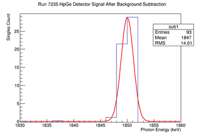
Then subtract
TH1F *coin1=new TH1F("coin1","coin1",30,1800,1860);

ntuple->Draw("ADC7*0.604963-49.7001 >>coin1")

TH1F *lin1=new TH1F("lin1","line1",30,1800,1860);

for(int i=1800;i<1861;i++){
lin1->Fill(i,-2028+1.12*i)
}

TH1F *sub1=new TH1F("sub1","sub1",30,1800,1860);

sub1->Add(coin1,1);
sub1->Add(lin1,-1);

sub1->Draw();
A pdf of the Mathematica notebook used to calculate background area, gaussian area, and plot signal/noise vs. activity.
File:AW Background Noise custom4.pdf
All the ROOT fit parameters used to find the background and the resulting peaks.
File:Y-88 Fit Log Scaled&Cut.pdf
Integrating the gaussian of the HpGe detector signal.
File:AW Gaussian Integral2.pdf
Old Analysis Section
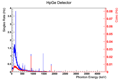
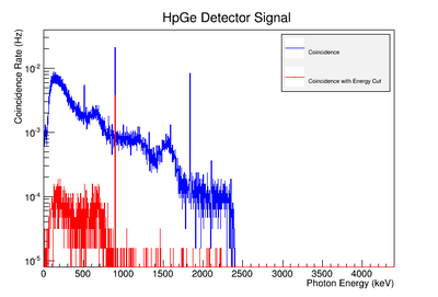
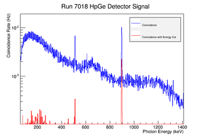
Using our Y-88 source, our set-up allows us to perform runs with the detectors in coincidence (AND mode) or singles (OR mode). The figure on the left shows the HpGe detector's coincidence events (red) that occurred within a 200 ns timing window. This graph has been overlaid with the same detector’s single events (blue). We can see that by having the detectors in coincidence, the noise is reduced and several peaks, which do not have multiple photons in coincidence, are removed.
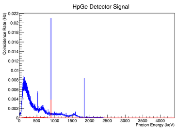
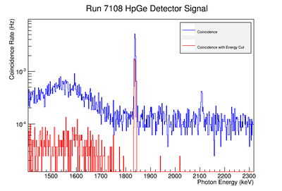
The coincidence run does not show the two energy peaks associated with Y-88 decay alone. Even though we require coincidence for the system to trigger, there is still noise. These peaks could be Compton events contaminating the coincidence and accidentals. Photons can loss a portion of their energy traveling to the detector. They do not necessarily have to deposit all of their energy into the detector either. The photon can Compton scatter out. It is not possible to tell the difference between a photon that deposited all of its energy from a scattered photon, since the speed of light is so fast and the resolution of the detector so poor. The photons can, however, be distinguished if an energy cut is applied. In order to remove the Compton events and the accidentals, we can require the photon energy to be completely deposited into the detector. This can be achieved by placing an energy cut on the NaI detector around the high energy Y-88 peak. This will remove other unwanted photon energies. The graph on the right is an overlay of the coincidence signal before (blue) and after (red) an energy cut is applied to the companion detector (NaI detector). The noise seen at low energies is greatly reduced after including the cut and improved the signal.
Background subtraction
898 keV analysis
The raw Histograms and fits may be found here A_W_thesis_old#898_keV_signal_table
The Measured half life is
| Days | Trig | Integral | Statistical Error | Systematic Error | Systematic Error without Coincidence Energy Cut | |
| 108 | 1.01 | sing | 1.364 | N/A | ||
| coin | 0.0052 | |||||
| 159 | 1.49 | sing | 0.8697 | N/A | ||
| coin | 0.0042 | |||||
| 229 | 2.15 | sing | 0.4733 | N/A | ||
| coin | 0.0034 | |||||
| 245 | 2.30 | sing | 0.5807 | N/A | ||
| coin | 0.0015 |
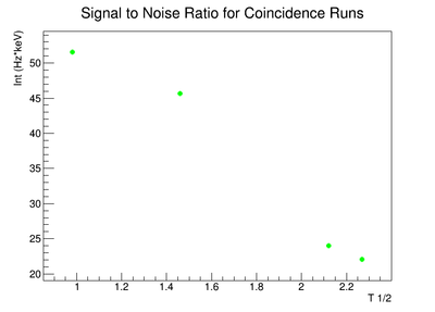
The signal to noise ratio is
| Days | Trig | SNR | Statistical Error | Systematic Error | |
| 108 | 1.01 | sing | 4.368 | ||
| coin | 46.181 | ||||
| 159 | 1.49 | sing | 8.228 | ||
| coin | 37.30 | ||||
| 229 | 2.15 | sing | 4.478 | ||
| coin | 30.195 | ||||
| 245 | 2.30 | sing | 5.494 | ||
| coin | 37.994 |
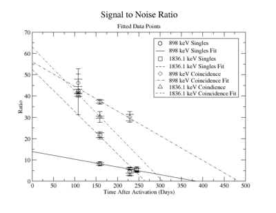
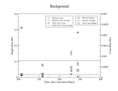
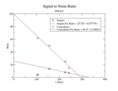
The first data point for the singles 898 keV was not included in the signal to noise fit. At the time of measurement, the noise was larger. This could be from contaminates with short half-lives in the sample that decayed away. Only elements with longer half-lives, such as Y-88, remained. The background of the remaining three data points were averaged.
For the 898 keV coincidence signal to noise fit, the last data point was not included. The length of the run and activities in the room, such as the nitrogen tank refilling, during counting caused the peak to be spread over a larger energy range. This also meant that the background noise would be larger. The background of the first three data points were averaged.
what about third data point
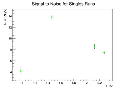
The following plot is the signal to noise ratio with only the data points used to obtain a fit.
| Energy | Trig | (days) | (before efficiency) (Hz) | (before efficiency) (nuclei) | (after efficiency) (Hz) | (after efficiency) (nuclei) | (days) | (Hz) | (nuclei) | |
| 898 | sing | 130.39 +/- 26.26 115.05 +/- 27.87 | 3.081 +/- 0.538 3.464 +/- 0.604 | 4.096e7 +/- 7.147e6 4.604e7 +/- 8.034e6 | 393.544 +/- 71.131 422.377 +/- 79.957 | 5.231e9 +/- 9.454e8 5.88e9 +/-1.063e9 | 383.63 | 32.506 +/- 18.162 36.539 +/- 20.416 | 4.320e8 +/- 2.414e8 4.857e8 +/- 2.714e8 | 0.0826 +/- 0.0485 |
| coin | 108.18 +/- 4.89 | 0.0154 +/- 0.0003 | 204958.085 +/- 4201.641 | 9.125 +/- 0.633 | 1.213e8 +/- 8.416e6 | 483.60 | 0.3935 +/- 0.0951 | 5.230e6 +/- 1.264e6 | 0.0431 +/- 0.0108 | |
| 1836.1 | sing | 106.16 +/- 8.63 | 2.317 +/- 0.262 | 3.080e7 +/- 3.480e6 | 742.929 +/- 87.053 | 9.874e9 +/- 1.157e9 | 264.94 | 132.74 +/- 20.938 | 1.764e9 +/- 2.783e8 | 0.1787 +/- 0.0351 |
| coin | 100.10 +/- 4.0 | 0.0196 +/- 0.0004 | 260440.778 +/- 5339.036 | 10.033 +/- 0.447 | 1.334e8 +/- 5.946e6 | 305.63 | 1.376 +/- 0.298 | 1.829e7 +/- 3.958e6 | 0.1371 +/- 0.0303 |
March 2015
| Energy | Trig | (days) | (before efficiency) (Hz) | (before efficiency) (nuclei) | (after efficiency) (Hz) | (after efficiency) (nuclei) | (days) | (Hz) | (nuclei) | |
| 898 | sing | 152.83 +/- 26.99 | 1.371 +/- 0.239 | 1.822e7 +/- 3.180e6 | 175.093 +/- 31.647 | 2.327e9 +/- 4.206e8 4.057e9 +/- 7.333e8 | ||||
| coin | 108.18 +/- 4.89 | 0.0154 +/- 0.0003 | 204958.085 +/- 4201.641 | 9.125 +/- 0.633 | 1.213e8 +/- 8.416e6 | 483.60 | 0.3935 +/- 0.0951 | 5.230e6 +/- 1.264e6 | 0.0431 +/- 0.0108 | |
| 1836.1 | sing | 101.099 +/- 14.473 | 0.904 +/- 0.102 | 1.202e7 +/- 1.358e6 | 289.993 +/- 33.98 | 3.854e9 +/- 4.516e8 5.471e9 +/- 6.410e8 | ||||
| coin | 100.10 +/- 4.0 | 0.0196 +/- 0.0004 | 260440.778 +/- 5339.036 | 10.033 +/- 0.447 | 1.334e8 +/- 5.946e6 | 305.63 | 1.376 +/- 0.298 | 1.829e7 +/- 3.958e6 | 0.1371 +/- 0.0303 |
Average :
- = number of atoms in sample that were activated
- = activity measure at time
- = photo nuclear cross section
- = photon flux
- = decay constant
- = irradiation time
- = decay time that has expired until A is measured
Using nickel target you can take ratios to try and approximate
Media:ContHealtPhys_Bevelacqua_2004APPIII.pdf
http://www.nist.gov/pml/data/xcom/
| Sample | (keV) | Activity (Hz) | Parent Nuclei (barn) | |
| Y-88 | 898 | 7.53e-8 | ||
| 1836.1 | ||||
| Ni-57 | 1377.63 | 1.188 | 5.41e-6 | |
| 511 | ||||
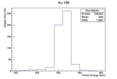
| Au-196 | 355.73 | 5.886 | 1.30e-6 | |
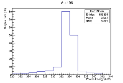
| 333.03 |
- = 5 hr =18000 s
- = 5 days = 432000 s
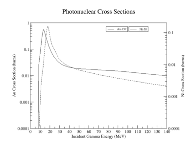
File:Photonuclear xsections.pdf
Nickel normalization
Reaction
Run list
Photon absorption cross sections:
Ni-58 plot data table
Ni-60 http://www.nndc.bnl.gov/sigma/getPlot.jsp?evalid=15652&mf=3&mt=5&nsub=0
Ni-61 http://www.nndc.bnl.gov/sigma/getPlot.jsp?evalid=15653&mf=3&mt=5&nsub=0
Ni-62 http://www.nndc.bnl.gov/sigma/getPlot.jsp?evalid=15654&mf=3&mt=5&nsub=0
Ni-64 http://www.nndc.bnl.gov/sigma/getPlot.jsp?evalid=15655&mf=3&mt=5&nsub=0
according to pg 13.3 on gets the total cross section by adding up the cross section in the tables up to the desired energy.
http://www.bnl.gov/isd/documents/70393.pdf
Gold normalization
Reaction:
Naturally occurring Isotopes of Gold are Au-197 ( 100% )
Neutron knockout:
Au-197 ->Au-196 has the following lines in order of decreasing intensity: 355.73, 333.03 , half life =9.6 hours, 6.167 days
Proton knockout:
Goes to a stable isotope
NP knockout:
Au-197->Pt-195 no high intensity lines above 100 keV , half life = 4.010 days
Photon absorption cross sections:
Au-197
1836.1 Analysis
The raw Histograms and fits may be found here A_W_thesis_old#1836_keV_signal_table
The Measured half life is
| Days | Trig | Integral | Statistical Error | Systematic Error | Systematic Error without Coincidence Energy Cut | |
| 108 | 1.01 | sing | 0.8414 | N/A | ||
| coin | 0.0062 | |||||
| 159 | 1.49 | sing | 0.5015 | N/A | ||
| coin | 0.0046 | |||||
| 229 | 2.15 | sing | 0.2822 | N/A | ||
| coin | 0.0062 | |||||
| 245 | 2.30 | sing | 0.2449 | N/A | ||
| coin | 0.0016 |
The signal to noise ratio is
| Days | Trig | SNR | Statistical Error | Systematic Error | |
| 108 | 1.01 | sing | 42.07 | ||
| coin | 40.666 | ||||
| 159 | 1.49 | sing | 21.52 | ||
| coin | 30.172 | ||||
| 229 | 2.15 | sing | 4.64 | ||
| coin | 40.666 | ||||
| 245 | 2.30 | sing | 5.43 | ||
| coin | 0.7569 |
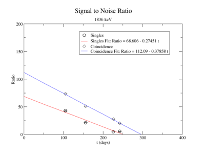
For the 1836 keV coincidence signal to noise fit, the last data point was not included. The length of the run and activities in the room, such as the nitrogen tank refilling, during counting caused the peak to be spread over a larger energy range. This also meant that the background noise would be large. The background of the first three data points were averaged.
The following plot is the signal to noise ratio with only the data points used to obtain a fit.
| Energy | Trig | (days) | (before efficiency) (Hz) | (before efficiency) (nuclei) | (after efficiency) (Hz) | (after efficiency) (nuclei) | (days) | (Hz) | (nuclei) | |
| 898 | sing | 130.39 +/- 26.26 | 3.081 +/- 0.538 | 4.096e7 +/- 7.147e6 | 393.544 +/- 71.131 | 5.231e9 +/- 9.454e8 | 383.63 | 32.506 +/- 18.162 | 4.320e8 +/- 2.414e8 | 0.0826 +/- 0.0485 |
| coin | 108.18 +/- 4.89 | 0.0154 +/- 0.0003 | 204958.085 +/- 4201.641 | 9.125 +/- 0.633 | 1.213e8 +/- 8.416e6 | 483.60 | 0.3935 +/- 0.0951 | 5.230e6 +/- 1.264e6 | 0.0431 +/- 0.0108 | |
| 1836.1 | sing | 106.16 +/- 8.63 | 2.317 +/- 0.262 | 3.080e7 +/- 3.480e6 | 742.929 +/- 87.053 | 9.874e9 +/- 1.157e9 | 264.94 | 132.74 +/- 20.938 | 1.764e9 +/- 2.783e8 | 0.1787 +/- 0.0351 |
| coin | 100.10 +/- 4.0 | 0.0196 +/- 0.0004 | 260440.778 +/- 5339.036 | 10.033 +/- 0.447 | 1.334e8 +/- 5.946e6 | 305.63 | 1.376 +/- 0.298 | 1.829e7 +/- 3.958e6 | 0.1371 +/- 0.0303 |
Average :
Error analysis
1.) rate energy cuts
2.) Energy calibration error
3.) Linear background fit error
4.) Gaussian integration of Signal - background peak
5.) ignorable error from run length time
6.) Coincidence energy cut.
7.) dividing by average background for SNR
8.) correction ratio for 3rd data point
9.) error in half life to find N0 for the detection limit extrapolation
10.) error extrapolation efficiency to higher energy lines for N0 calculation
Energy Window systematic error
The signal is measured by subtracting a count rate that is summed over an energy interval. The choice of this integration interval, energy window, is a source of systematic error. In order to calculate the error associated with the energy window, its range was adjusted based on the statistical variance of the background subtracted count rate fit to a gaussian. The integral was measured for window ranges chosen according to an integer interval of the standard deviation , where n = 3,4,5. The difference between the largest and mid-value was taken as the positive standard deviation, and the lowest was used for the standard deviation negative fluctuation. The resulting errors were divided by the signal to obtain a percent error as shown in column 1 of TableXXX.
Energy calibration systematic error
Prior to each measurement of the Y-88 sample's activity, the detectors where calibrated using several standard sources with known activity and dominant energy lines. This was accomplished by counting certified samples of Cs-137, Co-60, and Na-22 as well as Ba-133 and Mn-54. The observed mean ADC channel number was correlated with the expected energy line from each of the above sources. The correlation was measured using a standard linear fit algorithm. The linear fit algorithm determines the uncertainty of each fit parameter, the slope and the y-intercept. The effects of this uncertainty on the signal was analysed and is referred to as the energy calibration error.
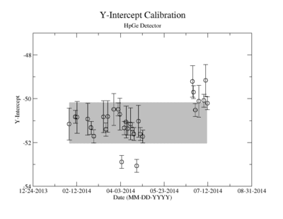
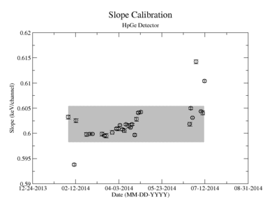
The uncertainty in the energy calibration just before a singles measurement was used to investigate the impact of the calibration on the measured signal for a given energy window of integration. While the singles measurements took less than 10 minutes, the coincidence measurement required more than 24 hours. The long term variance of the energy calibration shown in Figure ZZ.XXX was used to estimate the impact of the energy calibration drift during the coincidence measurements. The fit's y-intercept has a temporal variance corresponding to a relative uncertainty of about 1.865%; the slope is about 0.608%. The effects of this error on the coincidence signal were analysed. In both cases, the range of the energy widow is held constant while the slope and the y-intercept where adjusted to account for all possible combinations with and without their respective uncertainty. The integral value was recorded after every fit parameter change and the max, min, and mean values were obtained. The difference between the largest and mean value was taken as the positive standard deviation, and the lowest was used for the standard deviation's negative fluctuation. The resulting errors were divided by the signal to obtain a percent error as shown in column 2 of TableXXX.
Linear Fit Systematic error
The signal is determine by subtracting the underlying background. A estimate of this background is made by fitting the observed count rate with the function below :
.
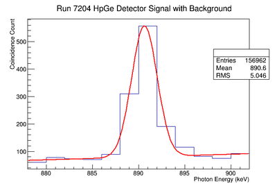
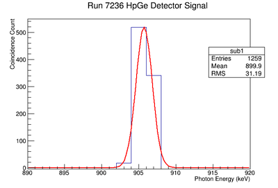
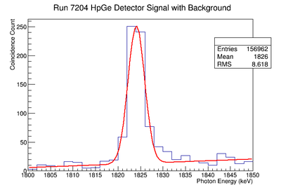
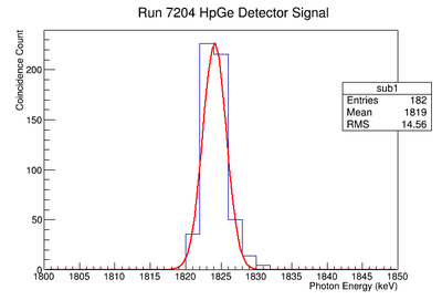
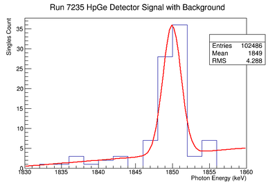
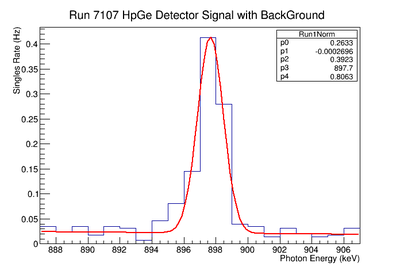
The above function contains a Gaussian representing the measured signal and a linear function for the background. The above figure XX.YY shows the fit applied. The linear fit parameters are used to create a histogram that is subtracted from the raw signal histogram, resulting in a histogram of just a signal. The energy window range used for the fit was adjusted and several fits performed to determine the uncertainty of the fit's slope and y-intercept. This systematic error, based on the fits dependence on the energy window is shown in the table under the column labeled "Linear Fit of Background". The fit parameters where adjusted to determine the maximum and minimum area of the background. For minimum background area, it was required that the area be positive. The difference between the maximum and unadjusted area value was taken as the positive standard deviation's fluctuation, and the minimum was used for the standard deviation's negative fluctuation. The resulting errors were divided by the signal to obtain a percent error as shown in column 3 of TableXXX.
Systematic error of the Coincidence Energy Cut
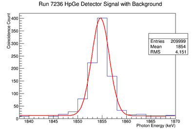
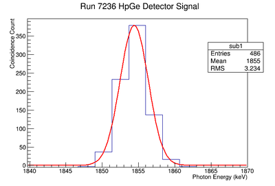
Figure AAA.XXX below show the coincidence measurements made before(blue) and after(red) energy cuts are applied on the NaI signal to reduce the accidental coincidence events and photons that fail to deposit all their energy in the NaI detector due to compton scattering.
To analyze the error association with coincidence counting only, the signal on the NaI detector was fit to a gaussian distribution. The of the gaussian fit was used to adjust the energy cut limits. The energy window was set at . The intergal values were recorded for each instance and the difference between the maximum and unadjusted integral values were taken as the positive standard deviation's fluctuation while the minimums were used for the standard deviation's negative fluctuation. The resulting errors were divided by the coincidence signal to obtain a percent error as shown in column 5 of TableXXX. The limited energy resolution of the NaI detector makes this uncertainty the dominant systematic error. If two HpGe detectors are used, then this uncertainty would decrease substantially will be far less than the remaining dominant systematic error; the energy Gaussian integral uncertainty. We report this systematic uncertainty but it is not propagated for the final result in order consider the case of a coincidence apparatus using two HpGe detectors.
Half-life
898 keV Singles
| Days | Trig | Energy Window | Energy Calibration | Linear Fit of Background | Gaussian Integration of Signal | Total Systematic Error | |
| 108 | 1.01 | sing | |||||
| 159 | 1.49 | sing | |||||
| 229 | 2.15 | sing | |||||
| 245 | 2.30 | sing |
898 keV Coincidence
| Days | Trig | Energy Window | Energy Calibration | Linear Fit of Background | Gaussian Integration of Signal | Coincidence Energy | Total Systematic Error | Systematic Error without Coincidence Energy Cut | |
| 108 | 1.01 | coin | |||||||
| 159 | 1.49 | coin | |||||||
| 229 | 2.25 | coin | |||||||
| 245 | 2.30 | coin |
1836.1 keV Singles
| Days | Trig | Energy Window | Energy Calibration | Linear Fit of Background | Gaussian Integration of Signal | Total Systematic Error | |
| 108 | 1.01 | sing | |||||
| 159 | 1.49 | sing | |||||
| 229 | 2.15 | sing | |||||
| 245 | 2.30 | sing |
1836.1 keV Coincidence
| Days | Trig | Energy Window | Energy Calibration | Linear Fit of Background | Gaussian Integration of Signal | Coincidence Energy Cut | Total Systematic Error | Systematic Error without Coincidence Energy Cut | |
| 108 | 1.01 | coin | |||||||
| 159 | 1.49 | coin | |||||||
| 229 | 2.15 | coin | |||||||
| 245 | 2.30 | coin |
Systematic error in the SNR
The singles measurement of the 898 keV peak had an initial high background that decays quickly and was more or less constant for singles measurements take 159 days after irradiation. We assumed that this reflected the presence of activated material with half lives longer that 245 days. As a result the background for the last three measurements was averaged and used in the denominator for the SNR. The first singles measurement has a large background due to activated nuclei with short half lives. This background decreased substantially after about 51 days when the next measurement was taken (the half-life of Y-88 is 106.6 days). The singles background near the 1836 keV line was measured to be around 0.5 Hz and fluctuated less over the experiment compared to the background around the 898 peak. The coincidence measurements had such little background, due to the nature of the apparatus, that the background was averaged over the first three measurements for both the 898 and the 1836 peaks separately. The background for the final coincidence measurements was ignored because of the increased noise produced when the detectors nitrogen dewar was filled during the 5 day background measurement.
The systematic uncertainty of the background was not analysed and propagated into the final SNR uncertainty. The signal's total systematic error, described above, was used for the final uncertainty.
Signal to Noise Ratio
| Energy (keV) | Trig | Variance of Averaged Background |
| 898 | sing | |
| coin | ||
| 1836.1 | sing | N/A |
| coin |
The background's systematic error is being ignored.
Background contribution to the SNR error
The analysis of the background uncertainty is described in the above section, "Linear Fit Systematic error." The background's relative statistical uncertainty shown in column 5 of TableXXX is calculated by varying the integral of the background by the uncertainties from the fit and dividing by the background used for the SNR ratio calculation. Column 6 presents the uncertainty of the averaged background as mentioned in the previous section. The variance the coincidence measurement is considerable larger than the individual coincidence measurements. The background in each singles measurement is smaller than the average variance indicating that the individual background measurements could have been made longer to improve their statistical uncertainty.
898 keV Background
| Days | Trig | Background | Linear Fit of Background Error | Statistical Error of Averaged Background | |
| 108 | 1.01 | sing | 0.3123 | N/A | |
| coin | 9.518e-5 | ||||
| 159 | 1.49 | sing | 0.0777 | ||
| coin | 8.732e-5 | ||||
| 229 | 2.15 | sing | 0.1532 | ||
| coin | 1.554e-4 | ||||
| 245 | 2.30 | sing | 0.0862 | ||
| coin | 3.948e-5 |
1836 keV Background
| Days | Trig | Background | Linear Fit of Background Error | Statistical Error | |
| 108 | 1.01 | coin | 1.037e-4 | ||
| 159 | 1.49 | coin | 4.248e-5 | ||
| 229 | 2.15 | coin | 3.112e-4 | ||
| 245 | 2.30 | coin | 2.114e-3 |
Singles Efficiency on 2/28/2014
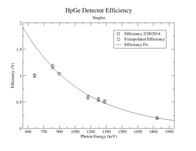
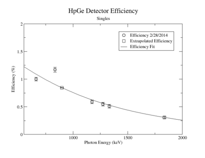
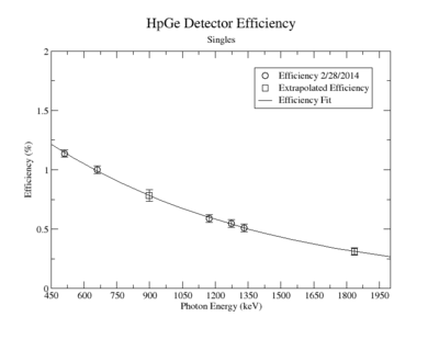
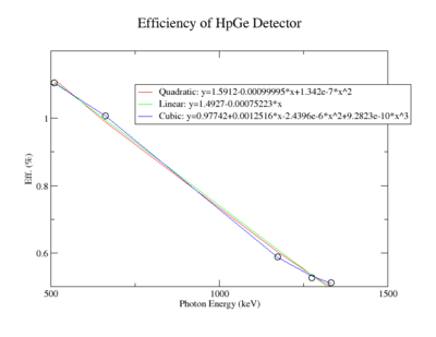
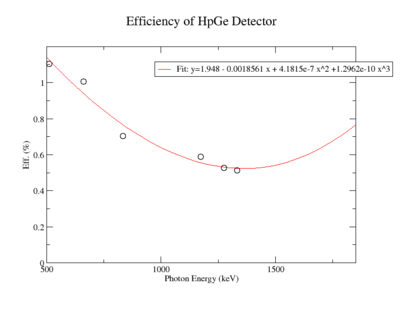
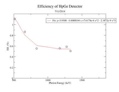
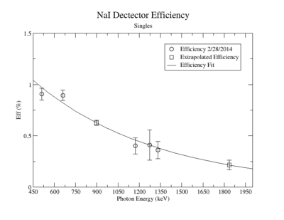
A measurement of the HpGe detectors geometric efficiency for detecting the Y-88 energy lines at 898 keV and 1836.1 keV was performed in order to determine the absolute activity of the sample. The count rate for several sources of known activity was measured by the data acquisition system. Since each sample has decayed since the original calibration by the source vendor, column 4 of tableXX.YY. reports the expected rates from each calibrated sample that were calculated using the half life and the known activity of the standard sources. The characteristic energy peaks from each source was fit to a gaussian distribution. The variance from that fit was used to determine the range of integration for the count rate measurement. The integration energy range was selected to include counts over the energy interval from to . The measured rates for each calibrated source using the HpGe detector are listed in column 5. The efficiency given by the ratio of the rates in column 5 to the expected rates in column 4 are shown in column 6 of the same table. The percent efficiency of the standard sources was fit to a exponential curve shown in figureXX.YY. The singles efficiency for 898 keV and 1836.1 keV were extrapolated from the exponential equation and are recorded in tableXX.YY. This process was repeated for the NaI detector and the results can be seen in figureXX.YY and tablesXX.YY and XX.YY.
HpGe Detector
| Run | Source | Energy | Expected rate (Hz) | HpGe Det B Rate (ADC 7) (Hz) | HpGe Eff (%) |
| 7027 | Na-22 | 511 | 1589.218 +/- 49.425 | 18.07 +/- 0.111 | 1.137 +/- 0.0317 |
| 7025 | Cs-137 | 661.657 | 2548.03 +/- 80.008 | 25.468+/- 0.172 | 0.9995 +/- 0.0321 |
| 7029 | Mn-54 | 834.848 | 41.405 +/- 1.300 | 0.485 +/- 0.014 | 1.171 +/- 0.0427 |
| 7026 | Co-60 | 1173.228 | 1876.619 +/- 58.926 | 11.03 +/- 0.106 | 0.588 +/- 0.0328 |
| 7027 | Na-22 | 1274.537 | 888.264 +/- 27.625 | 4.857 +/- 0.034 | 0.5468 +/- 0.0319 |
| 7026 | Co-60 | 1332.492 | 1878.167 +/- 58.974 | 9.584 +/- 0.023 | 0.510 +/- 0.0315 |
  1  Constant     6.36491e-01   4.70444e-02   1.00271e-05  -3.28621e-03
  2  Slope       -9.81232e-04   5.68236e-05   1.21109e-08  -1.59453e+00
Extrapolated Efficiency
| Source | Energy | HpGe Eff (%) |
| Y-88 | 898 | 0.7830 +/- 0.0471 |
| Y-88 | 1836.1 | 0.3119 +/- 0.0310 |
NaI Detector
| Run | Source | Energy | Expected rate (Hz) | NaI Det B Rate (ADC 7) (Hz) | NaI Eff (%) |
| 7027 | Na-22 | 511 | 1589.218 +/- 49.425 | 14.393 +/- 0.715 | 0.9057 +/- 0.0586 |
| 7025 | Cs-137 | 661.657 | 2548.03 +/- 80.008 | 22.8 +/- 0.9154 | 0.8948 +/- 0.0510 |
| 7026 | Co-60 | 1173.228 | 1876.619 +/- 58.926 | 7.529 +/- 0.5503 | 0.4012 +/- 0.0796 |
| 7027 | Na-22 | 1274.537 | 888.264 +/- 27.625 | 3.654 +/- 0.5266 | 0.4114 +/- 0.1474 |
| 7026 | Co-60 | 1332.492 | 1878.167 +/- 58.974 | 6.784 +/- 0.5345 | 0.3612 +/- 0.0848 |
| Source | Energy | NaI Eff (%) |
| Y-88 | 898 | 0.6262 +/- 0.0246 |
| Y-88 | 1836.1 | 0.2158 +/- 0.0466 |
Coincidence Efficiency
Unlike the singles efficiency found above, the efficiency for a coincidence measurement relies on the combined efficiency of both detectors. A known Y-88 source was not available to measure the coincidence activity directly. Instead, the HpGe's geometric efficiency for detecting the Y-88 energy lines at 898 keV and 1836.1 keV was combined with the NaI detectors efficiency for the 1836.1 and 898 keV lines respectively. For example, to obtain the 898 keV coincidence efficiency, the HpGe singles efficiency at this energy line is multiplied by the NaI singles efficiency at the 1836.1 keV line. The uncertainties of the singles efficiency are added in quadrature and the resulting values recorded in column 4 of tableXX.YY. The reverse case was applied to find the coincidence efficiency at the 1836.1 keV line and the values are listed in column 4 of tableXX.YY.
| Source | HpGe Singles 898 keV Eff (%) | NaI Singles 1836.1 keV Eff (%) | HpGe Coincidence Eff (%) |
| Y-88 | 0.7830 +/- 0.0471 | 0.2158 +/- 0.0466 | 0.1690 +/- 0.0663 |
| Source | HpGe Singles 1836.1 keV Eff (%) | NaI Singles 898 keV Eff (%) | HpGe Coincidence Eff (%) |
| Y-88 | 0.3119 +/- 0.0310 | 0.6262 +/- 0.0246 | 0.1953 +/- 0.0396 |


