Advanced Nuclear Physics
References:
Krane:
Catalog Description:
PHYS 609 Advanced Nuclear Physics 3 credits.
Nucleon-nucleon interaction, bulk nuclear structure,
microscopic models of nuclear structure, collective
models of nuclear structure, nuclear decays
and reactions, electromagnetic interactions, weak
interactions, strong interactions, nucleon structure,
nuclear applications, current topics in nuclear
physics. PREREQ: PHYS 624 OR PERMISSION
OF INSTRUCTOR.
PHYS 624-625 Quantum Mechanics 3 credits.
Schrodinger wave equation, stationary state
solution; operators and matrices; perturbation
theory, non-degenerate and degenerate cases;
WKB approximation, non-harmonic oscillator,
etc.; collision problems. Born approximation,
method of partial waves. PHYS 624 is a PREREQ
for 625. PREREQ: PHYS g561-g562, PHYS 621
OR PERMISSION OF INSTRUCTOR.
Click here for Syllabus
Introduction
The interaction of charged particles (electrons and positrons) by the exchange of photons is described by a fundamental theory known as Quantum ElectroDynamics. QED has perturbative solutions which are limited in accuracy only by the order of the perturbation you have expanded to. As a result the theory is quite useful in describing the interactions of electrons that are prevalent in Atomic physics.
Nuclear physics, however, encompasses the physics of describing not only the nucleus of an Atom but also the composition of the nucleons (protons and neutrons) which are the constituent of the nucleus. Quantum ChromoDynamic (QCD) is the fundamental theory designed to describe the interactions of the quarks and gluons inside a nucleon. Unfortunately, QCD does not have a complete solution at this time. At very high energies, QCD can be solved perturbatively. This is an energy [math]E[/math] at which the strong coupling constant [math]\alpha_s[/math] is less than unity where
- [math]\alpha_s \approx \frac{1}{\beta_o \ln{\frac{E^2}{\Lambda^2_{QCD}}}}[/math]
- [math]\Lambda_{QCD} \approx 200 MeV[/math]
The "Standard Model" in physics is the grouping of QCD with Quantum ElectroWeak theory. Quantum ElectroWeak theory is the combination of Quantum ElectroDynamics with the weak force; the exchange of photons, W-, and Z-bosons.
The objectives in this class will be to discuss the basic aspects of the nuclear phenomenological models used to describe the nucleus of an atom in the absence of a QCD solution.
Nomenclature
| Variable |
Definition
|
| Z |
Atomic Number = number of protons in an atom
|
| A |
Atomic Mass
|
| N |
number of neutrons in an atom = A-Z
|
| Nuclide |
A specific nuclear species
|
| Isotope |
Nuclides with same Z but different N
|
| Isotones |
Nuclides with same N but different Z
|
| Isobars |
Nuclides with same A
|
| Nuclide |
A specific nuclear species
|
| Nucelons |
Either a neutron or a proton
|
| J |
Nuclear Angular Momentum
|
| [math]\ell[/math] |
angular momentum quantum number
|
| s |
instrinsic angular momentum (spin)
|
| [math]\vec{j}[/math] |
total angular momentum = [math]\vec{\ell} + \vec{s}[/math]
|
| [math]Y_{\ell,m_{\ell}}[/math] |
Spherical Harmonics, [math]\ell[/math] = angular momentum quantum number, [math]m_{\ell}[/math] = projection of [math]\ell[/math] on the axis of quantization
|
| [math]\hbar[/math] |
Planks constant/2[math]\pi = 6.626 \times 10^{-34} J \cdot s / 2 \pi[/math]
|
Notation
[math]{A \atop Z} X_N[/math] = An atom identified by the Chemical symbol [math]X[/math] with [math]Z[/math] protons and [math]N[/math] neutrons.
Notice that [math]Z[/math] and [math]N[/math] are redundant since [math]Z[/math] can be identified by the chemical symbol [math]X[/math] and [math] N[/math] can be determined from both [math]A[/math] and the chemical symbol [math]X[/math](N=A-Z).
- example
- [math]{208 \atop\; }Pb ={208 \atop 82 }Pb_{126}[/math]
Historical Review
Rutherford Nuclear Atom (1911)
Rutherford
interpreted the experiments done by his graduate students Hans Geiger and Ernest Marsden involving scattering of alpha particles by the thin gold-leaf. By focusing on the rare occasion (1/20000) in which the alpha particle was scattered backward, Rutherford argued that most of the atom's mass was contained in a central core we now call the nucleus.
Chadwick discovers neutron (1932)
Prior to 1932, it was believed that a nucleus of Atomic mass [math]A[/math] was composed of [math]A[/math] protons and [math](A-Z)[/math] electrons giving the nucleus a net positive charge [math]Z[/math]. There were a few problems with this description of the nucleus
- A very strong force would need to exist which allowed the electrons to overcome the coulomb force such that a bound state could be achieved.
- Electrons spatially confined to the size of the nucleus ([math]\Delta x \sim 10^{-14}m = 10 \;\mbox{fermi})[/math] would have a momentum distribution of [math]\Delta p \sim \frac{\hbar}{\Delta x} = 20 \frac{\mbox {MeV}}{\mbox {c}}[/math]. Electrons ejected from the nucleus by radioactive decay ([math]\beta[/math] decay) have energies on the order of 1 MeV and not 20.
- Deuteron spin: The total instrinsic angular momentum (spin) of the Deuteron (A=2, Z=1) would be the result of combining two spin 1/2 protons with a spin 1/2 electron. This would predict that the Deuteron was a spin 3/2 or 1/2 nucleus in contradiction with the observed value of 1.
The discovery of the neutron as an electrically neutral particle with a mass 0.1% larger than the proton led to the concept that the nucleus of an atom of atomic mass [math]A[/math] was composed of [math]Z[/math] protons and [math](A-Z)[/math] neutrons.
Powell discovers pion (1947)
Although Cecil Powell is given credit for the discovery of the pion, Cesar Lattes is perhaps more responsible for its discovery. Powell was the research group head at the time and the tradition of the Nobel committe was to award the prize to the group leader. Cesar Lattes asked Kodak to include more boron in their emulsion plates making them more sensitive to mesons. Lattes also worked with Eugene Gardner to calcualte the pions mass.
Lattes exposed the plates on Mount Chacaltaya in the Bolivian Andes, near the capital La Paz and found ten two-meson decay events in which the secondary particle came to rest in the emulsion. The constant range of around 600 microns of the secondary meson in all cases led Lattes, Occhialini and Powell, in their October 1947 paper in 'Nature ', to postulate a two-body decay of the primary meson, which they called p or pion, to a secondary meson, m or muon, and one neutral particle. Subsequent mass measurements on twenty events gave the pion and muon masses as 260 and 205 times that of the electron respectively, while the lifetime of the pion was estimated to be some 10-8 s. Present-day values are 273.31 and 206.76 electron masses respectively and 2.6 x 10⁻⁸ s. The number of mesons coming to rest in the emulsion and causing a disintegration was found to be approximately equal to the number of pions decaying to muons. It was, therefore, postulated that the latter represented the decay of positively-charged pions and the former the nuclear capture of negatively-charged pions. Clearly the pions were the particles postulated by Yukawa.
In the cosmic ray emulsions they saw a negative pion (cosmic ray) get captured by a nucleus and a positive pion (cosmic ray) decay. The two pion types had similar tracks because of their similar masses.
Nuclear Properties
The nucleus of an atom has such properties as spin, mangetic dipole and electric quadrupole moments. Nuclides also have stable and unstable states. Unstable nuclides are characterized by their decay mode and half lives.
Decay Modes
| Mode |
Description
|
| Alpha decay |
An alpha particle (A=4, Z=2) emitted from nucleus
|
| Proton emission |
A proton ejected from nucleus
|
| Neutron emission |
A neutron ejected from nucleus
|
| Double proton emission |
Two protons ejected from nucleus simultaneously
|
| Spontaneous fission |
Nucleus disintegrates into two or more smaller nuclei and other particles
|
| Cluster decay |
Nucleus emits a specific type of smaller nucleus (A1, Z1) smaller than, or larger than, an alpha particle
|
| Beta-Negative decay |
A nucleus emits an electron and an antineutrino
|
| Positron emission(a.k.a. Beta-Positive decay) |
A nucleus emits a positron and a neutrino
|
| Electron capture |
A nucleus captures an orbiting electron and emits a neutrino - The daughter nucleus is left in an excited and unstable state
|
| Double beta decay |
A nucleus emits two electrons and two antineutrinos
|
| Double electron capture |
A nucleus absorbs two orbital electrons and emits two neutrinos - The daughter nucleus is left in an excited and unstable state
|
| Electron capture with positron emission |
A nucleus absorbs one orbital electron, emits one positron and two neutrinos
|
| Double positron emission |
A nucleus emits two positrons and two neutrinos
|
| Gamma decay |
Excited nucleus releases a high-energy photon (gamma ray)
|
| Internal conversion |
Excited nucleus transfers energy to an orbital electron and it is ejected from the atom
|
Time
Time scales for nuclear related processes range from years to [math]10^{-20}[/math] seconds. In the case of radioactive decay the excited nucleus can take many years ([math]10^6[/math]) to decay (Half Life). Nuclear transitions which result in the emission of a gamma ray can take anywhere from [math]10^{-9}[/math] to [math]10^{-12}[/math] seconds.
Units and Dimensions
| Variable |
Definition
|
| 1 fermi |
[math]10^{-15}[/math] m
|
| 1 MeV |
=[math]10^6[/math] eV = [math]1.602 \times 10^{-13}[/math] J
|
| 1 a.m.u. |
Atomic Mass Unit = 931.502 MeV
|
Resources
The following are resources available on the internet which may be useful for this class.
Lund Nuclear Data Service
in particular
The Lund Nuclear Data Search Engine
Several Table of Nuclides
BNL
LANL
Korean Atomic Energy Research Institute
National Physical Lab (UK)
Quantum Mechanics Review
- Debroglie - wave particle duality
| Particle |
Wave
|
| [math]E[/math] |
[math]\hbar \omega = h \nu[/math]
|
| [math]P[/math] |
[math]\hbar k = \frac{h}{\lambda}[/math]
|
- Heisenberg uncertainty relationship
- [math]\Delta x \Delta p_x \ge \frac{\hbar}{2}[/math]
- [math]\Delta E \Delta t \ge \frac{\hbar}{2}[/math]
- [math]\Delta \ell_z \Delta \phi \ge \frac{\hbar}{2}[/math] where [math]\phi[/math] characterizes the location of [math]\ell[/math] in the x-y plane
- Classical: [math]\frac{p^2}{2m} + V(r) = E[/math]
- Quantum (Shrodinger Equation): [math]-\frac{\hbar^2}{2m}\nabla^2 \Psi + V(r) \Psi = i\hbar \frac{\partial \Psi}{\partial t}[/math]
- [math]\;\;\;\;\;\; p_x \rightarrow -i \hbar \frac{\partial}{\partial x} \;\;\; E \rightarrow i \hbar \frac{\partial}{\partial t}[/math]
- E = energy eigenvalues
- [math]\Psi(x,t) = \psi(x)e^{-\omega t}[/math] = eigenvectors [math]\omega=\frac{E}{\hbar}[/math]
- [math]P = \int_{x_1}^{x_2}\Psi^*(x,t) \Psi(x,t)[/math] = probability of finding the particle (wave packet) between [math]x_1[/math] and [math]x_2[/math]
- [math]\Psi^*[/math] = complex conjugate [math](i \rightarrow -i)[/math]
- [math]\lt f\gt = \int \Psi^* f \Psi dx =\lt \Psi^*| f| \Psi\gt [/math] = average (expectation) value of observable [math]f[/math] after many measurements of [math]f[/math]
- example: [math]\lt p_x\gt =\int \Psi^* \left ( -i\hbar \frac{\partial}{\partial x}\right ) \Psi dx[/math]
- Constraints on Quantum solutions
- [math]\psi[/math] is continuous accross a boundary : [math]\lim_{\epsilon \rightarrow 0} \left [ \psi(a+\epsilon) - \psi(a-\epsilon)\right ] =0[/math] and [math]\lim_{\epsilon \rightarrow 0} \left [ \left(\frac{\partial \psi}{\partial x} \right )_{a+\epsilon} - \left(\frac{\partial \psi}{\partial x} \right )_{a-\epsilon}\right ] =0[/math] ( if [math]V(x)[/math] is infinite this second condition can be violated)
- the solution is normalized:[math]\int \psi^* \psi dx =\lt \psi^* | \psi \gt =1[/math]
- Current conservation: the particle current density associated with the wave function \Psi is given by
- [math]j = \frac{\hbar}{2mi} \left ( \Psi^* \frac{\partial \Psi}{\partial x}-\Psi \frac{\partial \Psi^*}{\partial x}\right )[/math]
Schrodinger Equation
1-D problems
Free particle
If there is no potential field (V(x) =0) then the particle/wave packet is free. The wave function is calculated using the time-dependent Schrodinger equation:
- [math]-\frac{\hbar^2}{2m} \nabla^2 \Psi(x,t) + 0 = i\hbar\frac{\partial \Psi(x,t)}{\partial t}[/math]
Using separation of variables Let:
- [math]\Psi(x,t) = \psi(x) f(t)[/math]
Substituting we have
- [math]-\frac{\hbar^2}{2m} f(t) \frac{d^2 \psi(x)}{d x^2} = i \hbar \psi(x) \frac{d f(t)}{d t}[/math]
reorganizing you can move all functions of [math]x[/math] on one side and [math]t[/math] on the other suggesting that both sides equal some constant which we will call [math]E[/math]
- [math]-\frac{\hbar^2}{2m} \frac{1}{\psi(x)} \frac{d^2 \psi(x)}{d x^2} = i \hbar \frac{1}{f(t)} \frac{d f(t)}{d t} \equiv E[/math]
Solving the temporal (t) part:
- [math]\frac{1}{f(t)} \frac{d f(t)}{d t} = -\frac{i E}{\hbar} \Rightarrow f(t) = e^{-iEt/\hbar}[/math] : just integrate this first order diff eq.
Solving the spatial (x) part:
- [math]\frac{1}{\psi(x)} \frac{d^2 \psi(x)}{d x^2} =- \frac{2m E}{\hbar^2}[/math]
Such second order differential equations have general solutions of
- [math]\psi(x) = A e^{ikx} + B e^{-ikx}[/math] where [math]k^2 = \frac{2mE}{\hbar^2}[/math]
Now put everything together
- [math]\Psi(x,t) = \psi(x) f(t) = \left (A e^{ikx} + B e^{-ikx} \right ) e^{-iEt/\hbar}[/math]
- [math]= A e^{i(kx-\omega t)} + B e^{-i(kx-\omega t)}[/math]
- Notice
- [math]\lt \Psi(x,t) | \Psi(x,t)\gt = \lt \psi(x)| \psi(x)\gt \Rightarrow [/math]the wave function amplitude does not change with time
- also, if the operator for an observable A does not change in time, then
- [math]\lt \Psi(x,t) | A | \Psi(x,t)\gt = \lt \psi(x)| A| \psi(x)\gt \Rightarrow [/math] even though particles are not stationary they are in a quantum state which does not change with time (unlike decays).
- the term of amplitude[math] A[/math] represents a wave traveling in the +x direction while the second term represents a wave traveling in the -x direction.
- Example
- consider a free particle traveling in the +x direction
- Then
- [math]\Psi(x,t) = A e^{i(kx-\omega t)}[/math]
- if the particles are coming from a source at a rate of[math] j[/math] particles/sec then
- [math]j = \frac{\hbar}{2mi} \left ( \Psi^* \frac{\partial \Psi}{\partial x}-\Psi \frac{\partial \Psi^*}{\partial x}\right )[/math]
- [math]= \frac{\hbar}{2mi} \left ( A^*A[ik] - A A^* [-ik]\right ) = \frac{\hbar k}{m} \left ( A^*A\right )= \frac{\hbar k}{m} \left | A \right |^2[/math]
- [math]\Rightarrow A = \sqrt{\frac{mj}{\hbar k}}[/math]
Step Potential
Consider a 1-D quantum problem with the Step potential V(x) define below where [math]V_o \gt 0[/math]
- [math]V(x) =\left \{ {0 \;\;\;\; x \lt 0 \atop V_o \;\;\;\; x\gt 0} \right .[/math]
Break these types of problems into regions according to how the potential is defined. In this case there will be 2 regions
x<0
When x<0 then V =0 and we have a free particle system which has the solution given above.
- [math]\Psi_1(x,t) = \psi_1(x) f(t) = \left (A e^{ikx} + B e^{-ikx} \right ) e^{-iEt/\hbar}[/math]
- [math]= A e^{i(kx-\omega t)} + B e^{-i(kx-\omega t)}[/math] where [math]k^2 =\frac{2mE}{\hbar^2}[/math] and [math]\omega =\frac{E}{\hbar}[/math]
x>0
- [math]-\frac{\hbar^2}{2m} \nabla^2 \Psi_2(x,t) + V_o = i\hbar\frac{\partial \Psi_2(x,t)}{\partial t}[/math]
- [math]-\frac{\hbar^2}{2m} \frac{\partial^2 \Psi_2(x,t)}{\partial x^2} + V_o = i\hbar\frac{\partial \Psi_2(x,t)}{\partial t}[/math]
separation of variables: [math]\Psi_2(x,t) = \psi_2(x)f(t)[/math]
- [math]-\frac{\hbar^2}{2m} f(t)\frac{\partial^2 \psi_2(x)}{\partial x^2} + V_o\psi(x)f(t) = i\hbar \psi_2(x)\frac{\partial f(t)}{\partial t}[/math]
- [math]-\frac{\hbar^2}{2m} \frac{1}{\psi_2(x)}\frac{\partial^2 \psi_2(x)}{\partial x^2} + V_o = i\hbar \frac{1}{f(t)}\frac{\partial f(t)}{\partial t} \equiv E =[/math] Constant
The time dependent part of the problem is the same as the free particle solution. Only the spatial part changes because the Potential is not time dependent.
- [math]-\frac{\hbar^2}{2m} \frac{1}{\psi_2(x)}\frac{\partial^2 \psi_2(x)}{\partial x^2} =E - V_o = [/math] Constant
- [math] \frac{\partial^2 \psi_2(x)}{\partial x^2} =-\frac{2m}{\hbar^2}(E - V_o) \psi_2(x) [/math]
If [math]E \gt V_o[/math] then we have a wave that traverses the step potential partly reflected and partly transmitted, otherwise it will be reflected back and the part that is transmitted will tunnel through the barrier attenuated exponentially for x>0.
Here is how it works out mathematically
[math]E \gt V_o[/math]
For the case where [math]E \gt V_o[/math]:
- [math] \frac{\partial^2 \psi_2(x)}{\partial x^2} =-\frac{2m}{\hbar^2}(E - V_o) \psi_2(x) \equiv -k_2^2 \psi_2(x)\lt 0 [/math]
- [math] \frac{\partial^2 \psi_2(x)}{\partial x^2} \equiv -k_2^2 \psi_2(x)\lt 0 \Rightarrow[/math]SHM solutions
The above Diff. Eq. is the same form as the free particle but with a different constant
- Let
- [math]\psi_2(x) = Ce^{ik_2x} + De^{-ik_2x}[/math]
Now apply Boundary conditions:
- [math]\psi(x=0) = \psi_2(x=0)[/math]
- [math]A + B = C + D : e^{\pm i 0} = 1[/math]
and
- [math]\frac{\partial \psi}{\partial x}|_{x=0} = \frac{\partial \psi_2}{\partial x}|_{x=0}[/math]
- [math]k(A-B) = k_2 (C-D)[/math]
We now have a system of 2 equations and 4 unknowns which we can't solve.
- Notice
- The coefficient "D" in the above system represent the component of [math]\psi_2[/math] represent a wave moving from the right towards x=0. If we assume the free particle encountered this step potential by originating from the left side, then there is no way we can have a component of [math]\psi_2[/math] moving to the left. Therefore we set [math]D=0[/math].
- The coefficient A represent the incident plane wave on the barrier. The remaining coefficients B and C represent the reflected and transmitted components of the traveling wave, respectively.
- Know our system of equations is
- [math]A+B =C[/math]
- [math]A -B = \frac{k_2}{k} C[/math]
- If I assume that the coefficient A is known (I know what the amplitude of the incoming wave is) then I can solve the above system such that
- [math]A+B = C = (A-B)\frac{k}{k_2}[/math]
- [math]B=A\frac{1-\frac{k_2}{k}}{1+\frac{k_2}{k}}[/math]
similarly
- [math]C = A+B = A\left (1+ \frac{1-\frac{k_2}{k}}{1+\frac{k_2}{k}} \right ) = \frac{2A}{1+\frac{k_2}{k}}[/math]
Reflection (R) and Transmission (T) Coefficients
- [math]R\equiv \frac{j_{reflected}}{j_{incident}} = \frac{|B|^2}{|A|^2} = \left ( \frac{1-\frac{k_2}{k}}{1+\frac{k_2}{k}} \right )^2[/math]
- [math]T\equiv \frac{j_{transmitted}}{j_{incident}} = \frac{C^*ik_2C + Cik_2C^*}{A^*ikA + AikA^*} = \frac{k_2 |C|^2}{k |A|^2} =\frac{4 \frac{k_2}{k}}{\left ( 1 + \frac{k_2}{k} \right )^2} [/math]
- [math]=1 - R =1-\left ( \frac{1-\frac{k_2}{k}}{1+\frac{k_2}{k}} \right )^2 =\frac{ \left( 1+\frac{k_2}{k} \right )^2 - \left ( 1-\frac{k_2}{k}\right )^2}{\left ( 1+\frac{k_2}{k}\right )^2}=\frac{4 \frac{k_2}{k}}{\left ( 1 + \frac{k_2}{k} \right )^2} [/math]
[math]E \lt V_o[/math]
- [math] \frac{\partial^2 \psi_2(x)}{\partial x^2} =-\frac{2m}{\hbar^2}(E - V_o) \psi_2(x) \gt 0[/math]
- Let
- [math]k_3 \equiv \sqrt{\frac{2m}{\hbar^2}(V_o-E)}[/math]
Then
- [math] \frac{\partial^2 \psi_3(x)}{\partial x^2} =k_3 \psi_3(x) \gt 0 \Rightarrow[/math] exponential decay
- Assume solution
- [math]\psi_3 = G e^{k_3x} + Fe^{-k_3x}[/math]
- Recall the solution for x<0
- [math]\psi_1(x,t) = A e^{ikx} + B e^{-ikx}[/math] where [math]k^2 =\frac{2mE}{\hbar^2}[/math]
- Apply Boundary conditions
If [math]x \rightarrow \infty[/math]
Then [math]e^{\infty} \rightarrow \infty \Rightarrow G =0[/math]
- [math]\psi_3 = Fe^{-k_3x}[/math]
- Continuous conditions at x=0
- [math]A+B = F[/math]
- [math]ik(A-B) = -k_3F[/math]
Assuming A is known we have 2 equations and 2 unknowns again
- [math]A+B = \frac{ik}{-k_3} (A-B)[/math]
- [math]B=-A\left(\frac{1+\frac{ik}{k_3}}{1-\frac{ik}{k_3}} \right) = A\left(\frac{1-\frac{ik_3}{k}}{1+\frac{ik_3}{k}} \right)[/math]
- [math]F = A\left (1-\left(\frac{1-\frac{ik_3}{k}}{1+\frac{ik_3}{k}}\right) \right)=\frac{2A}{1+\frac{ik_3}{k}}[/math]
Reflection (R) and Transmission (T) Coefficients=
- [math]R\equiv \frac{j_{reflected}}{j_{incident}} = \frac{|B|^2}{|A|^2} = \left(\frac{1-\frac{ik_3}{k}}{1+\frac{ik_3}{k}} \right)\left(\frac{1-\frac{ik_3}{k}}{1+\frac{ik_3}{k}} \right)^*[/math]
- [math]=\left(\frac{1-\frac{ik_3}{k}}{1+\frac{ik_3}{k}} \right)\left(\frac{1-\frac{-ik_3}{k}}{1+\frac{-ik_3}{k}} \right) = 1[/math]
- [math]T\equiv \frac{j_{transmitted}}{j_{incident}} = \frac{F^*k_3F - Fk_3F^*}{A^*ikA + AikA^*} =0 =1-R [/math]
- Evanescent waves
- : Waves like [math]\psi_3[/math] which carry no current. There is a finite probability of penetrating the barrier (tunneling) but no net current is transmitted. A feature which separates Quantum mechanics from classical.
Rectangular Barrier Potential
Barrier potentials are 1-D step potentials of height (V_o > 0) which have a finite step width:
- [math]V(x) =0 \;\;\; x\lt 0[/math]
- [math]V(x) =\left \{ {V_o \;\;\;\; 0 \le x \le a \atop 0 \;\;\;\; x\gt a} \right .[/math]
We now have 3 regions in space to solve the schrodinger equation
We now from the free particle solutions that on the left and right side of the barrier we should have
- [math]\psi_1 = = A e^{ikx} + B e^{-ikx)} \;\;\; x \lt 0[/math]
- [math]\psi_3 = = F e^{ikx} + G e^{-ikx)} \;\;\; x \gt a[/math]
where
- [math]k^2= \frac{2mE}{\hbar^2}[/math]
But in the region [math]0 \le x \le a[/math] we have the save type of problem as the step in which the solution depends on the Energy of the system with respect to the potential. One solution for the [math]E\gt V_o[/math] (oscilatory) system and one for the [math]E\lt V_o[/math] (exponetial decay) system.
- [math]\psi_2 = \left \{ {= Ce^{ik_2x} + De^{-ik_2x} \;\;\;\; E\gt V_o \atop = Ce^{k_3x} + De^{-k_3x} \;\;\;\; E \lt V_o } \right .[/math]
where
- [math]k_2^2=\frac{2m(E-V_o)}{\hbar^2}\;\;\; k_3^2=\frac{2m(V_o-E)}{\hbar^2}[/math]
[math]E \gt V_o[/math]
For the case where [math]E \gt V_o[/math]:
Before we set [math]D =0[/math] because there wasn't a wave moving to the left towards the [math]x=0[/math] interface. The rectangular barrier though could have a wave reflect back form the [math]x=a[/math] interface.
- Apply Boundary conditions
- [math]\psi_1(x=0) = \psi_2(x=0)[/math]
- [math]A + B = C + D : [/math]
and
- [math]\psi_2(x=a) = \psi_3(x=a)[/math]
- [math]Ce^{ik_2a} + De^{-ik_2a} = Fe^{ika} + Ge^{-ika} [/math]
and
- [math]\frac{\partial \psi_1}{\partial x}|_{x=0} = \frac{\partial \psi_2}{\partial x}|_{x=0}[/math]
- [math]k(A-B) = k_2 (C-D)[/math]
and
- [math]\frac{\partial \psi_2}{\partial x}|_{x=a} = \frac{\partial \psi_3}{\partial x}|_{x=a}[/math]
- [math]k_2(Ce^{ik_2a}-De^{-ik_2a}) = k (Fe^{ika}-Ge^{-ika})[/math]
We now have a system of 4 equations
and 6 unknowns (A,B,C, D, F and G).
But:
- [math]G=0[/math] : no source for wave moving to left when x>a
If we treat [math]A[/math] as being known (you know the incident wave amplitude) then we have 4 unknowns (B,C,D, and F) and the 4 equations:
- [math]A + B = C + D : [/math]
- [math]k(A-B) = k_2 (C-D)[/math]
- [math]Ce^{ik_2a} + De^{-ik_2a} = Fe^{ika} : [/math]
- [math]k_2(Ce^{ik_2a}-De^{-ik_2a}) = k Fe^{ika}[/math]
Transmission
- [math]T \equiv \frac{|F|^2}{|A|^2}[/math] = the transmission coefficient
To find the ration of F to A
- solve the last 2 equations for C & D in terms of F
- solve the first 2 equations for A in terms C and D
- 3.)substitute your values for C and D from the last 2 equations so you have the ratio of B/A in terms of F/A
- 1.)solve the last 2 equations
- [math]Ce^{ik_2a} + De^{-ik_2a} = Fe^{ika} : [/math]
- [math]Ce^{ik_2a}-De^{-ik_2a} = \frac{k}{k_2} Fe^{ika}[/math]
for C and D
- [math]2Ce^{ik_2a} =Fe^{ika}\left ( 1+\frac{k}{k_2} \right)[/math]
- [math]2De^{-ik_2a} =Fe^{ika}\left ( 1-\frac{k}{k_2} \right)[/math]
- 2.) solve the first 2 equations for B in terms of C & D
- [math]A + B = C + D : [/math]
- [math]A-B = \frac{k_2}{k} (C-D)[/math]
for A in terms of C and D
- [math]2B=C \left ( 1- \frac{k_2}{k}\right ) + D\left ( 1+ \frac{k_2}{k}\right )[/math]
- [math]=\frac{F}{2}e^{i(k-k_2)a}\left ( 1+\frac{k}{k_2}\right ) \left ( 1- \frac{k_2}{k}\right ) +\frac{F}{2}e^{i(k+k_2)a}\left ( 1-\frac{k}{k_2} \right)\left ( 1+ \frac{k_2}{k}\right )[/math]
- [math]=\frac{F}{2}e^{i(k-k_2)a}\left ( \frac{k}{k_2}-\frac{k_2}{k}\right ) +\frac{F}{2}e^{i(k+k_2)a}\left ( - \frac{k}{k_2}+\frac{k_2}{k}\right )[/math]
- [math]\Rightarrow \frac{B}{A} = \frac{Fe^{ika}}{4A}\left[ \left ( e^{-ik_2a} -e^{ik_2a}\right ) \frac{k}{k_2} +\left ( -e^{-ik_2a} -e^{ik_2a}\right ) \frac{k_2}{k} \right ][/math]
- [math]= -\frac{Fe^{ika}}{4A} \left [ 2i\sin(k_2a) \frac{k}{k_2} -2 i\sin(k_2a)\frac{k_2}{k}\right ][/math]
- 3.) Find Reflection Coeff in terms of Transmission Coeff
- [math]\frac{B}{A}=- \frac{F}{A}\frac{ie^{ika}\sin(k_2a)}{2} \left [ \frac{k^2-k_2^2}{kk_2} \right ][/math]
- [math]T +R = \frac{|F|^2}{|A|^2} + \frac{|B|^2}{|A|^2} = \frac{|F|^2}{|A|^2} + \frac{F^*}{A^*}\frac{-ie^{-ika}\sin(k_2a)}{2} \left [ \frac{k^2-k_2^2}{kk_2} \right ]\frac{F}{A}\frac{ie^{ika}\sin(k_2a)}{2} \left [ \frac{k^2-k_2^2}{kk_2} \right ] = 1[/math]
- [math]\Rightarrow \frac{|F|^2}{|A|^2} \left (1 + \frac{\sin^2(k_2a)}{4}\left [ \frac{k^2-k_2^2}{kk_2} \right ]^2 \right) = 1[/math]
or
- [math]T = \frac{|F|^2}{|A|^2} = \frac{1}{\left (1 + \frac{\sin^2(k_2a)}{4}\left [ \frac{k^2-k_2^2}{kk_2} \right ]^2 \right) }[/math]
since
- [math]k^2= \frac{2mE}{\hbar^2} \;\;k_2^2= \frac{2m(E-V_o)}{\hbar^2}[/math]
Then
- [math]T = \frac{|F|^2}{|A|^2} = \frac{1}{\left (1 + \frac{\sin^2(k_2a)}{4}\left [ \frac{V_o^2}{E(E-V_o)} \right ] \right) }[/math]
3-D problems
Infinite Spherical Well
What is the solution to Schrodinger's equation for a potential V which only depends on the radial distance (r) from the origin of a coordinate system?
- [math]V =\left \{ {0 \;\;\;\; r\lt a \atop \infty \;\;\;\; r\gt a} \right .[/math]
Such a potential lends itself to the use of a Spherical coordinate system in which the schrodinger equation has the form
- [math]\hat{H}\psi(r,\theta,\phi) = E\psi(r,\theta,\phi)[/math]
- [math]-\frac{\hbar^2}{2m}\nabla^2 \psi(r,\theta,\phi)+V\psi(r,\theta,\phi) = E\psi(r,\theta,\phi)[/math]
In spherical coordinates
- [math]\nabla^2 = \frac{1}{r} \frac{\partial^2}{\partial r^2} r + \frac{1}{r^2} \left ( \frac{1}{\sin(\theta)} \frac{\partial}{\partial \theta} \sin(\theta)\frac{\partial}{\partial \theta} + \frac{1}{\sin^2(\theta)}\frac{\partial^2}{\partial \phi^2}\right )[/math]
- Note
- [math]\frac{1}{r} \frac{\partial^2}{\partial r^2} r = \frac{1}{r} \frac{\partial}{\partial r} r \left ( \frac{1}{r} \frac{\partial}{\partial r} \right ) = \left (\frac{1}{r} \frac{\partial}{\partial r} \right)^2 \equiv -\left ( \frac{\hat{p}_r}{\hbar} \right )^2[/math]
- [math]\left ( \frac{1}{\sin(\theta)} \frac{\partial}{\partial \theta} \sin(\theta)\frac{\partial}{\partial \theta} + \frac{1}{\sin^2(\theta)}\frac{\partial^2}{\partial \phi^2}\right ) \equiv -\frac{\hat{L}^2}{\hbar^2}[/math]
so
- [math]\hat{H}\psi(r,\theta,\phi) = \left ( \frac{\hat{p}_r^2}{2m} + \frac{\hat{L}^2}{2mr^2} + V \right ) \psi(r,\theta,\phi)= E\psi(r,\theta,\phi)[/math]
Using separation of variables:
- [math]\psi(r,\theta,\phi) \equiv R(r) \Theta(\theta) \Phi(\phi)[/math]
which we can also write as
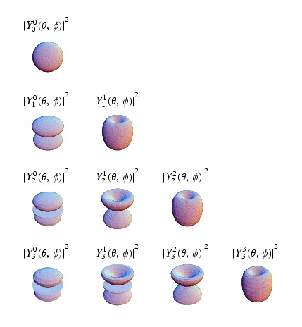
- [math]\psi(r,\theta,\phi) \equiv R(r) Y_{l,m}(\theta, \phi)[/math]
where
- [math]Y_{l,m}(\theta, \phi) \equiv \Theta(\theta) \Phi(\phi)[/math]
Substitute
- [math]\frac{1}{2mR(r)} \hat{p}_r^2 R(r)+ \frac{1}{2mr^2Y_{l,m}} \hat{L}^2 Y_{l,m}= E-V[/math]
V=0
We have a constant on the right hand side so the left hand side must also be constant
- [math]\frac{1}{2mr^2Y_{l,m}} \hat{L}^2 Y_{l,m} = \frac{l(l+1)\hbar^2}{2mr^2} =[/math]a "centrifugal" barrier which keeps particles away from r=0
substituting
- [math]\frac{1}{2mR(r)} \hat{p}_r ^2R(r) + \frac{l(l+1)\hbar^2}{2mr^2} = E-V[/math]
In the region where V=0
- [math]\frac{1}{\hbar^2R(r)}\hat{p}_r^2 R(r) + \frac{l(l+1)}{r^2} = \frac{2m}{\hbar^2}E[/math]
The Radial equation becomes
- [math]\left ( \frac{\hat{p}_r^2}{\hbar^2}+ \frac{l(l+1)}{r^2} \right ) R(r)= \left ( \frac{-1}{r} \frac{\partial^2}{\partial r^2} r + \frac{l(l+1)}{r^2} \right ) R(r)=\frac{2mE}{\hbar^2}R(r)[/math]
Let
- [math]k^2 = \frac{2mE}{\hbar^2}[/math]
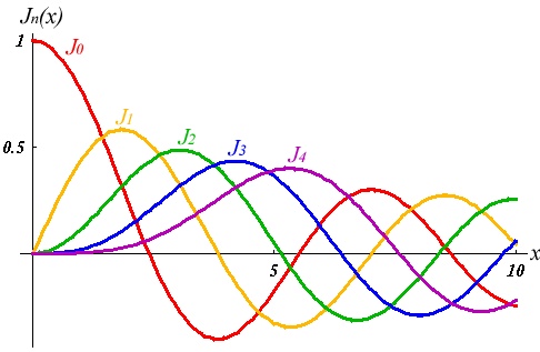
Then we have the "spherical Bessel"differential equation with the solutions:
- [math]j_l(kr) = \left (\frac{-r}{k} \right ) ^l \left (\frac{1}{r} \frac{d}{dr} \right )^l j_o (kr)[/math]
where
- [math]j_o(kr) = \frac{sin(kr)}{kr}[/math]
[math]Y_{l,m}[/math] and [math] j_l[/math] Table
| [math]l[/math] |
[math] m_l [/math] |
[math] j_l[/math] |
[math]Y_{l,m_l}[/math]
|
| 0 |
0 |
[math]\frac{\sin(kr)}{kr} = \frac{1}{2ikr} \left ( e^{ikr}-e^{-ikr} \right)[/math] |
[math]\sqrt{\frac{1}{4 \pi}}[/math]
|
| 1 |
0 |
[math]\frac{\sin(kr)}{(kr)^2} -\frac{\cos(kr)}{kr}[/math] |
[math]\sqrt{\frac{3}{4 \pi}}\cos(\theta)[/math]
|
|
[math]\pm[/math] 1 |
|
[math]\mp \sqrt{\frac{3}{8 \pi}}\sin(\theta)e^{\pm i \phi}[/math]
|
| 2 |
0 |
[math]\left ( \frac{3}{(kr)^3} - \frac{1}{kr} \right )\sin(kr) -\frac{3\cos(kr)}{(kr)^2}[/math] |
[math]\sqrt{\frac{5}{16 \pi}}(3\cos^2(\theta)-1)[/math]
|
|
[math]\pm[/math] 1 |
|
[math]\mp \sqrt{\frac{15}{8 \pi}}\sin(\theta)\cos(\theta)e^{\pm i \phi}[/math]
|
|
[math]\pm[/math] 2 |
|
[math]\mp \sqrt{\frac{15}{32 \pi}}\sin^2(\theta)e^{\pm 2 i \phi}[/math]
|
The general solution for the 3-D spherical infinite potential well problem is
- [math]\psi_{k,l,m}(r,\theta,\phi) = j_l(kr) Y_{l,m}(\theta, \phi)[/math] = eigen function(s)
where
- [math]k,l,m[/math] are quantization number and [math]E_k = \frac{\hbar^2 k^2}{2m} =[/math] quantum energy level = eigen state(s)
Energy Levels
To find the Energy eignevalues we need to know the value for "k". We apply the boundary condition
- [math]j_l(kr)= 0 [/math] at [math]r=a[/math]
to determine the "nodes" of [math]j_l[/math]; ie value of [math]ka[/math] so if you tell me the size of the well then I can tell you the value of k which will satisfy the boundary conditions. This means that "k" is not a "real" quantum number in the sense that it takes on integral values.
We simple label states with an integer [math](n)[/math] representing the [math]n^{th}[/math] zero crossing via:
- [math]| n,l\gt = j_l(ka) Y_{l,m_l}[/math]
For example:
- In the [math] l =0[/math] case
- [math]j_o(ka) =\frac{sin(ka)}{ka} = 0 [/math]when [math](ka) = \pi, 2\pi, 3\pi, 4\pi, ...[/math]
- You arbitrarily label these state as [math]n=1 \Rightarrow (ka) =\pi \;\;\;\; k = \pi/a \;\;\;\;\; E_0=\frac{\hbar^2 (\pi)^2}{2ma^2}, n=2 \Rightarrow (ka) = 2\pi [/math]
- [math]|1,0\gt = j_o(\pi r/a) Y_{0,0} \;\;\; E=E_0[/math]
- [math]|2,0\gt = j_o(2\pi r/a) Y_{0,0};\;\; E=2^2E_0 = 4E_0[/math]
- [math]|3,0\gt = j_o(3\pi r/a) Y_{0,0};\;\; E=3^2E_0=9E_0[/math]
- [math]|4,0\gt = j_o(4\pi r/a) Y_{0,0};\;\; E=4^2E_0=16E_0[/math]
- In the [math] l =1[/math] case
- [math]|1,1\gt = j_1(4.49 r/a) Y_{1,m_l}\;\;\; E=\left(\frac{4.49}{\pi}\right )^2E_0=2.04E_0[/math]
- [math]|2,1\gt = j_1(7.73 r/a) Y_{1,m_l}\;\;\; E=\left(\frac{7.73}{\pi}\right )^2E_0=6.05E_0[/math]
- [math]|3,1\gt = j_1(10.9 r/a) Y_{1,m_l}\;\;\; E=\left(\frac{10.9}{\pi}\right )^2E_0=12.04E_0[/math]
- [math]|4,1\gt = j_1(14.07 r/a) Y_{1,m_l}\;\;\; E=\left(\frac{14.07}{\pi}\right )^2E_0=20.1E_0[/math]
- Notice
- The angular momentum is degenerate for each level making the degeneracy for each energy [math]= 2l+1[/math]
File:EnergyLevel3-DInfinitePotentialWell.jpg
Simple Harmonic Oscillator
The potential for a Simple Harmonic Oscillator (SHM) is:
- [math]V(r) = \frac{1}{2} kr^2[/math]
This potential is does not depend on any angles. It's a central potential. Our solutions for Y_{l,m} from the 3-D infinite well potential will work for the SHM potential as well! All we need to do is solve the radial differential equation:
- [math]\frac{1}{R(r)}\hat{p}_r^2 R(r) + \frac{l(l+1)}{r^2} = \frac{2m}{\hbar^2}\left ( E - \frac{1}{2} kr^2 \right )[/math]
- [math]\left ( \frac{-1}{r} \frac{\partial^2}{\partial r^2} r + \frac{l(l+1)}{r^2} \right ) R(r)= \frac{2m}{\hbar^2}\left ( E - \frac{1}{2} kr^2 \right )R(r)[/math]
or
- [math]\frac{\partial^2}{\partial r^2} R(r) +\frac{2}{r} \frac{\partial}{\partial r} R(r) + \left ( \frac{2m}{\hbar^2}\left ( E - \frac{1}{2} kr^2 \right) -\frac{l(l+1)}{r^2}\right ) R(r)= 0[/math]
When solving the 1-D harmonic oscillator solutions were found which contained the term [math]e^{-r^2/2}[/math]
Assume R(r) may be written as
- [math]R(r) = G(r) e^{-r^2/2}[/math]
substituting this into the differential equation gives
- [math]\frac{\partial^2 G}{\partial r^2} + \left ( \frac{2}{r} - \alpha r\right ) \frac{\partial G}{\partial r} + \left ( \lambda - \beta - \frac{l(l+1)}{r^2}\right ) G(r)= 0[/math]
The above differential equation can be solved using a power series solution
- [math]G = \sum_i^\infty a_ir^i[/math]
After performing the power series solution; ie find a recurrance relation for the coefficents a_i after substituting into the differential equation and require the coefficent of each power of r to vanish.
You arrive at a soultion of the form
- [math]\psi(r,\theta,\phi) \equiv R(r) Y_{l,m}(\theta, \phi) = e^{-r^2/2} G_{l,n} Y_{l,m}(\theta, \phi) [/math]
where
- [math]\ G_{l,n} =[/math] polynomial in [math]r[/math] of degree [math]n[/math] in which the lowest term in [math]r[/math] is [math]r^l[/math]
these polynomials are solutions to the differential equation
- [math]r^2\frac{\partial^2 G}{\partial r^2} + 2\left ( r-r^3\right ) \frac{\partial G}{\partial r} + \left ( 2nr^2- l(l+1)\right ) G(r)= 0[/math]
if you do the variable substitution
- [math]t = r^2[/math]
you get
- [math]t\frac{\partial^2 S}{\partial t^2} + \left ( l + \frac{3}{2} -t \right ) \frac{\partial S}{\partial t} + k S= 0[/math]
the above differential equation is called the "associated" Laguerre differential equation with the Laguerre polynomials as its solutions.
The following table gives you the Radial wave functions for a few SHO states:
| [math]n[/math] |
[math] l[/math] |
[math]E_n (\hbar \omega_o )[/math] |
[math]R(r)[/math]
|
| 0 |
0 |
[math]\frac{3}{2} [/math] |
[math]= \frac{2 \alpha^{3/2}}{\pi^{1/4}} e^{- \alpha^2 r^2/2}[/math]
|
| 1 |
1 |
[math]\frac{5}{2} [/math] |
[math]= \frac{2\sqrt{2} \alpha^{3/2}}{\sqrt{3} \pi^{1/4}} \alpha r e^{- \alpha^2 r^2/2}[/math]
|
| 2 |
0 |
[math]\frac{7}{2} [/math] |
[math]= \frac{2\sqrt{2} \alpha^{3/2}}{\sqrt{3} \pi^{1/4}} (\frac{3}{2} -\alpha^2 r^2 e^{- \alpha^2 r^2/2}[/math]
|
| 2 |
2 |
|
[math]= \frac{4 \alpha^{3/2}}{\sqrt{15} \pi^{1/4}} \alpha^2 r^2 e^{- \alpha^2 r^2/2}[/math]
|
| 3 |
1 |
[math]\frac{9}{2} [/math] |
[math]= \frac{4 \alpha^{3/2}}{\sqrt{15} \pi^{1/4}} (\frac{5}{2} \alpha r -\alpha^3 r^3 e^{- \alpha^2 r^2/2}[/math]
|
- Note
- Again there is a degeneracy of [math]2l+1[/math] for each [math]l[/math]
- Again E is independent of [math]l[/math] (central or constant potentials)
- if [math]n[/math] is odd [math]l[/math] is odd and if [math]n[/math] is even[math] l[/math] is even
- multiple values of [math]l[/math] occur for a give [math]n[/math] such that [math]l \le n[/math]
- The degeneracy is [math]\frac{1}{2} (n+1) (n+2)[/math] because of the above points
The Coulomb Potential for the Hydrogen like atom
The Coulomb potential is defined as :
- [math]V(r) = -\frac{Ze^2}{4 \pi \epsilon_0 r} [/math]
where
- [math]Z =[/math] atomic number
- [math]e =[/math] charge of an electron
- [math]\epsilon_0=[/math] permittivity of free space = [math]8.85 \times 10^{-12} Coul^2/(N m^2)[/math]
This potential is does not depend on any angles. It's a central potential. Our solutions for Y_{l,m} from the 3-D infinite well potential will work for the Coulomb potential as well! All we need to do is solve the radial differential equation:
- [math]\frac{1}{R(r)}\hat{p}_r^2 R(r) + \frac{l(l+1)}{r^2} = \frac{2m}{\hbar^2}\left ( E + \frac{k}{r} \right )[/math]
- [math]\left ( \frac{-1}{r} \frac{\partial^2}{\partial r^2} r + \frac{l(l+1)}{r^2} \right ) R(r)= \frac{2m}{\hbar^2}\left ( E + \frac{k}{r} \right )R(r)[/math]
or
- [math]\frac{1}{r}\frac{\partial^2}{\partial r^2} rR(r) + \left ( \frac{2m}{\hbar^2}\left ( E + \frac{k}{r} \right) -\frac{l(l+1)}{r^2}\right ) R(r)= 0[/math]
Radial Equation
Use the change of variable to alter the differential equiation
Let
- [math]G(r) \equiv r R(r)[/math]
Then the differential equation becomes:
- [math]\frac{\partial^2}{\partial r^2} G(r) + \left ( \frac{2m}{\hbar^2}\left ( E + \frac{k}{r} \right) -\frac{l(l+1)}{r^2}\right ) G(r)= 0[/math]
Consider the case where [math]|V| \gt |E| \Rightarrow[/math] (Bound states)
Bound state also imply that the eigen energies are negative
- [math]E = - |E|[/math]
Let
- [math]\kappa^2 \equiv \frac{2m |E|}{\hbar^2}[/math]
- [math]\rho \equiv 2 \kappa r[/math]
- [math]\lambda \equiv \left ( \frac{Ze^2 m }{\kappa \hbar^2} \right ) = Z \sqrt{\frac{\mathcal{R}}{|E|}}[/math]
- [math]\mathcal{R} = \frac{me^4}{2\hbar^2} = \frac{\hbar^2}{2m a_o^2} =1.09737316 \times 10^7\frac{1}{m} =[/math] Rydberg's constant
- [math]a_o = \frac{\hbar^2}{me^2} = 5.291772108 \times 10^{-11} m= 52918 fm =[/math] Bohr Radius
- [math]\frac{\partial^2}{\partial \rho^2} G(r) - \frac{l(l+1)}{\rho^2}G(r) + \left ( \frac{\lambda}{\rho} -\frac{1}{4} \right) G(r)= 0[/math]
Boundary conditions
- if [math]\rho[/math] is large then the diff equation looks like
- [math]\frac{\partial^2}{\partial \rho^2} G(r) -\frac{1}{4} G(r)= 0[/math]
- [math]\Rightarrow G(r) \sim Ae{-\rho/2} + B e^{\rho/2}[/math]
To keep[math] G(r \rightarrow \infty )[/math] finite at large [math]\rho[/math] you need to have B=0
- if \rho is very small ( particle close to the origin) then the diff equation looks like
- [math]\frac{\partial^2}{\partial \rho^2} G(r) - \frac{l(l+1)}{\rho^2} G(r)= 0[/math]
The general solution for this type of Diff Eq is
- [math]G(r) = \frac{A}{\rho^l} + B \rho^{l+1}[/math]
where A =0 so [math]G(r \rightarrow 0)[/math] is finite
A general solution is formed using a linear combination of these asymptotic solutions
- [math]G(r) = e^{-\rho/2} \rho^{l+1} F(\rho)[/math]
where
- [math]F(\rho) = \sum_{i=0}^{\infty} C_i \rho^i[/math]
substitute this power series solution into the differential equation gives
- [math]\rho \frac{d^2 F}{d \rho^2} + (2l + 2 - \rho) \frac{d F}{d \rho} - (l +1 - \lambda)F =0[/math]
which is again the associated Laguerre differential equation with a general series solution containing functions of the form
- [math]F(\rho) \sim e^{\rho}[/math]
with the recurrance relation
- [math]C_{i+1} = \frac{i+l+1 - \lambda}{(i+1)(i+2l+2)} C_i[/math]
notice that
- [math]G(r) = e^{-\rho/2} \rho^{l+1} e^{\rho}[/math]
now diverges for large [math]\rho[/math].
To keep the solution from diverging as well we need to truncate the coefficients[math] C_{i+1}[/math] at some [math] i_{max}[/math] by setting the coefficient to zero when
- [math]i_{max} = \lambda -l -1[/math]
This value of [math]\lambda[/math] for the truncations identifies a quantum state according to the integer [math]\lambda[/math] which truncates the solution and gives us our energy eigenvalues
- [math]\lambda^2 = \frac{Z^2 \mathcal{R}}{|E|}[/math]
or since \lambda is just a dummy variable
- [math]E_n = - |E_n| = -\frac{Z^2 \mathcal{R}}{n^2}[/math]
Coulomb Eigenfunctions and Eigenvalues
| [math]n[/math] |
[math] l[/math] |
Spec Not. |
[math]E_n (-\frac{Z^2 \mathcal{R}}{n^2} )= 13.6 eV[/math] |
[math]R(r)[/math]
|
| 1 |
0 |
1S |
[math]\frac{1}{1} [/math] |
[math]=2 \left ( \frac{Z}{a_o} \right)^{3/2} e^{- Z r/a_o}[/math]
|
| 2 |
1 |
2S |
[math]\frac{1}{4} [/math] |
[math]= \left ( \frac{Z}{2a_o} \right)^{3/2} (2 - Zr/a_o) e^{- Z r/2a_o}[/math]
|
| 2 |
1 |
2P |
[math]\frac{1}{4} [/math] |
[math]= \left ( \frac{Z}{2a_o} \right)^{3/2} \frac{Zr}{\sqrt{3}a_o} e^{- Z r/2a_o}[/math]
|
| 3 |
0 |
3S |
[math]\frac{1}{9} [/math] |
[math]= \left ( \frac{Z}{3a_o} \right)^{3/2} \left [ 2 - \frac{4Zr}{3 a_o} + 4 \left (\frac{Zr}{3\sqrt{3} a_o} \right)^2 \right ] e^{- Z r/3a_o}[/math]
|
| 3 |
1 |
3P |
[math]\frac{1}{9} [/math] |
[math]= \frac{4\sqrt{2}}{9} \left ( \frac{Z}{3a_o} \right)^{3/2} \left ( \frac{Zr}{a_o} \right) \left ( 1-\frac{Zr}{6a_o} \right ) e^{- Z r/3a_o}[/math]
|
| 3 |
2 |
3D |
[math]\frac{1}{9} [/math] |
[math]= \frac{2\sqrt{2}}{27\sqrt{5}} \left ( \frac{Z}{3a_o} \right)^{3/2} \left ( \frac{Zr}{a_o} \right)^2 e^{- Z r/3a_o}[/math]
|
The SHO and Coulomb schrodinger equations have Laguerre polynomial solutions for the radial part with the SHO solution polynomials of [math]r^2[/math] and the Coulomb solution polynomials linear in [math]r[/math]. The number of degenerate quantum states differs though, the SHO has 10 degenerate states while the Coulomb potential has 9 states.
Angular Momentum
Parity
Transitions
Dirac Equation
Nuclear Properties
Nuclear Radius
Binding Energy
Angular Momentum and Parity
The Nuclear Force
Yukawa Potential
Nuclear Models
Shell Model
Nuclear Decay and Reactions
Alpha Decay
Beta Decay
Gamma Decay
Electro Magnetic Interactions
Weak Interactions
Strong Interaction
Applications
Homework problems
NucPhys_I_HomeworkProblems

