Wire angle correspondance

Determining wire-theta correspondence

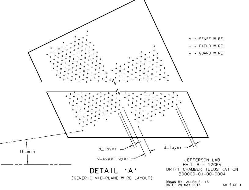
To associate the hits with the Moller scattering angle theta, the occupancy plots of the drift chamber hits by means of wire numbers and layer must be translated using the physical constraints of the detector. Using the data released for the DC:

DC: Drift Chambers(specs)

DC Geometry(geom)

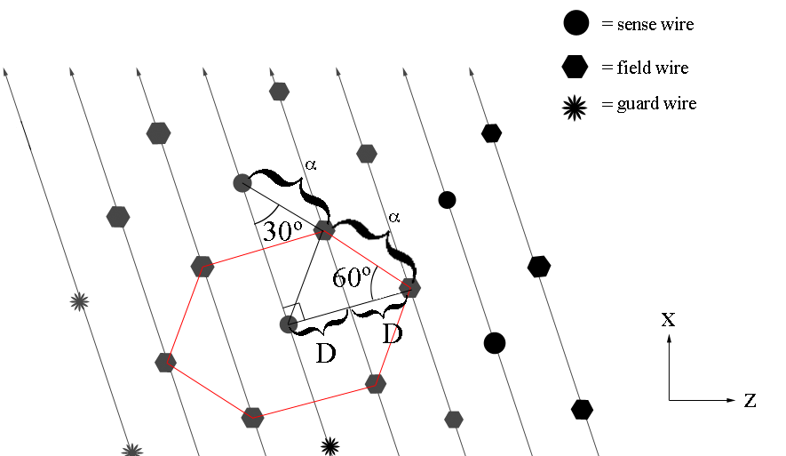
Examining the geometry file, we can see that each plane, not just the plane of the sense wires, is separated by a distance of D=.3861 cm. We can use the geometry of the wire placements to find

[math]\alpha=\frac{D}{\cos(60^{\circ})}=2D[/math]

Finding the separation distance between two adjacent sense wires

[math]d=4(.3861\ cm)\cos(30^{\circ})=1.337\ cm[/math]

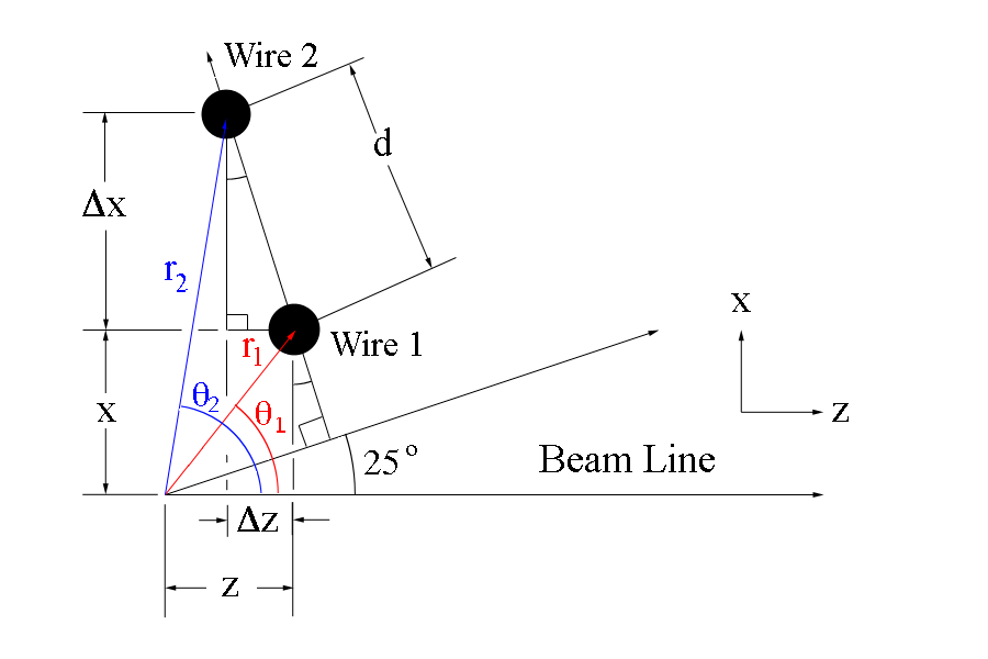
Since the separation between adjacent sense wires is uniform and at a set angle of 25 degrees with respect to the beam line, we can use this fact to determine the angle theta each wire makes when measured from the vertex.

[math]\Delta\ x=1.337\cos(25^{\circ})cm=1.212cm[/math]

[math]\Delta\ z=-1.337\sin(25^{\circ})cm=-0.5652cm[/math]

The new x and z coordinates for wire 2 can be found using the change in the components

[math]x'=x+\Delta x[/math] [math]z'=z+\Delta z[/math]

This can be extended to any point along the same wire plane, starting from the coordinates for wire 1

[math]x'=x+\Delta x\times\ n[/math] [math]z'=z+\Delta z\times\ n[/math]

The angle theta that the wire makes with the vertex is given by

[math]\tan{\theta}=\frac{x+\Delta x}{z+\Delta z}\Rightarrow \theta=\arctan{\frac{x+\Delta x}{z+\Delta z}}[/math]

CED Verification

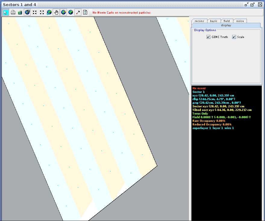
Using CED to verify the angle and wire correlation,

Zooming in on the view paralell to the direction of the wires in ced, we can examine the wire corresponding theta angle in the drift chamber.

Table 1: Superlayer 1 Wire 1 Coordinates

Coordinates(cm)	Layer 1	Layer 2	Layer 3	Layer 4	Layer 5	Layer 6
x	20.42	21.51	21.39	22.49	22.37	23.47
y	0.00	0.00	0.00	0.00	0.00	0.00
z	243.41	244.18	245.51	246.28	247.62	248.38

Table 2: Superlayer 1 Wire 2 Coordinates

Coordinates(cm)	Layer 1	Layer 2	Layer 3	Layer 4	Layer 5	Layer 6
x	21.64	22.73	22.61	23.71	23.58	24.69
y	0.00	0.00	0.00	0.00	0.00	0.00
z	242.86	243.62	244.94	245.71	247.05	247.81

Corresponding theta angles can be found for other wires, in Region 1, Superlayers 1 and 2.

Table 3: Superlayer 1 Wire-Angle Theta Correspondence in Degrees

Wire Number	Layer 1	Layer 2	Layer 3	Layer 4	Layer 5	Layer 6
1	4.79	5.03	4.98	5.22	5.16	5.40
2	5.09	5.33	5.27	5.51	5.45	5.69
62	24.42
63	24.76
64	25.10
77	29.46	29.60	29.41	29.55	29.37	29.51
78	29.79	29.93	29.74	29.88	29.69	29.83
79	30.12	30.26	30.07	30.21	30.02	30.16
110	40.19	40.28	40.05	40.13	39.91	39.99
111	40.51	40.59	40.36	40.44	40.21	40.29
112	40.82	40.90	40.67	40.75	40.52	40.60

Table 4: Superlayer 2 Wire-Angle Theta Correspondence in Degrees

Wire Number	Layer 1	Layer 2	Layer 3	Layer 4	Layer 5	Layer 6
1	4.79	5.03	4.98	5.22	5.16	5.40
2	5.09	5.33	5.27	5.51	5.45	5.69
77	29.46	29.60	29.41	29.56	29.37	29.51
78	29.79	29.93	29.74	29.88	29.70	29.84
79	30.13	30.27	30.07	30.21	30.02	30.16
110x	40.19	40.28	40.05	40.13	39.91	39.99
111	40.51	40.59	40.36	40.44	40.22	40.30
112	40.82	40.90	40.67	40.75	40.52	40.60

Super Layer 1:Layer 1

Table 1: Superlayer 1 Change of Coordinates From Wire 1 to Wire 2(cm)

Coordinates(cm)	Layer 1	Layer 2	Layer 3	Layer 4	Layer 5	Layer 6
[math]\Delta x[/math]	1.22	1.22	1.22	1.22	1.21	1.22
[math]\Delta y[/math]	0.00	0.00	0.00	0.00	0.00	0.00
[math]\Delta z[/math]	.55	.56	.57	.57	.57	.57

Using the geometric construction for determining angle theta to wire 2:

[math]\tan{\theta}=\frac{x+\Delta x}{z+\Delta z}\Rightarrow \theta=\arctan{\frac{x+\Delta x}{z+\Delta z}}[/math]

[math]\arctan{\frac{20.42+1.212}{243.39-0.5652}}=\arctan{\frac{21.632}{242.8248}}=\arctan{0.0891}=5.09^{\circ}[/math]

This equation can be solved for a hypothetical wire 0, which will allow the wire number to be the multiplicative factor for the change from the starting position.

[math]\tan{\theta}=\frac{x-\Delta x+n\Delta x}{z-\Delta z+n\Delta z}\Rightarrow \theta=\arctan{\frac{x'+n\Delta x}{z'+n\Delta z}}[/math]

where

[math]x'=20.42-1.212\approx 19.21cm[/math] [math]z'=243.39+0.5652\approx 243.96cm[/math]

[math]\theta=\arctan{\frac{19.21+n1.212}{243.39-n0.5652}}[/math]

Using Mathematica, a series expansion about n=0 can be found:

In[1]:= Series[ArcTan[(19.21+1.212 x)/(243.39-0.5652 n)],{n,0,4}]

Out[1]= 0.0787635+0.00513098 n+9.83726*10^-6 n^2-2.61675*10^-8 n^3-2.22826*10^-10 n^4+O[n]^5

[math]\theta\approx 0.0787635+0.00513098 n+9.83726\times 10^{-6} n^2-2.61675\times 10^{-8} n^3[/math]

This expression will find the angle theta in radians given the wire number. To convert from radians to degrees, we can multiply by 180 and divide by Pi.

In[2]:= 180*(0.07876354504106763`+0.005130982891104289` n+9.837257652182922`*^-6 n^2-2.616751708660921`*^-8 n^3-2.2282595631625944`*^-10 n^4+O[n]^5)/3.14159625359

Out[2]= 4.51281+0.293983 n+0.000563633 n^2-1.49929*10^-6 n^3-1.2767*10^-8 n^4+O[n]^5

[math]\theta\approx 4.51281+0.293983 n+0.000563633 n^2-1.49929\times10^{-6} n^3[/math]

This tells us that the expression for theta will follow a function that comes from a series expansion. To account for instrument and measurement errors, angle measurements from ced can be used to find a better fit.

Using Mathematica, a line can be fitted to the data collected on the wire number to angle theta correspondence.

Declaring the data set:

In[1]:= data1={{1,4.79},{2,5.09},{78,29.79},{111,40.50},{112,40.82}}

Out[1]= {{1,4.79},{2,5.09},{78,29.79},{111,40.5},{112,40.82}}

Testing for a linear fit:

In[2]:= line1=Fit[data1,{1,n},n]

Out[2]= 4.45395 +0.324738 n

Examing the range limits for the angle theta for layer 1:

Taking the difference of the upper and lower limits in theta,

[math]\Delta degrees=40.82^{\circ}-4.79^{\circ}=36.03^{\circ}[/math]

Dividing by the change in wire numbers (112-1=111), we find

[math]\frac{\Delta degrees}{\Delta wire\ number}=\frac{36.03^{\circ}}{111\ wires}\approx\ \frac{0.325^{\circ}}{wire\ number}[/math]

This would imply that if the wires were evenly placed, their change in angle theta would increase by the factor of .325 degrees for each increase in wire number, starting obviously with wire 1 at 4.79 degrees. In addition, this implies that the bin spacing for each wire would be around .325 degrees in width.

Chercking this, we can find the difference between wires 1 and 2,

[math]\frac{\Delta degree}{\Delta wire\ number}=\frac{5.09^{\circ}-4.79^{\circ} }{wire\ number}=\frac{.3^{\circ}}{wire\ number} [/math]

Similarly, finding the difference between wires 111 and 112,

[math]\frac{\Delta degree}{\Delta wire\ number}=\frac{40.82^{\circ}-40.51^{\circ}}{wire\ number}=\frac{.31^{\circ}}{wire\ number}[/math]

These differing values show that the bin width is not uniform in length, therefore a first order, linear fit, will not suffice.

Testing for a quadratic fit:

In[3]:= quad1=Fit[data1,{1,n,n^2},n]

Out[3]= 4.45253 +0.325072 n-3.05048*10^-6 n^2

The quadratic fit does not work since it's first derivative

[math]\theta'\approx \Delta \theta=.325072-6.83308\ n[/math]

does not give the same spacing between low and high values of n as seen in the ced data. The coefficient near the first order will have to smaller than .31 to find a correlation that would agree.

Testing for a polynomial of degree 3 fit:

In[118]:= polynomial1=Fit[data1,{1,n,n^2,n^3},n]

Out[118]= 4.48739 +0.300911 n+0.000510988 n^2-2.6919*10^-6 n^3

This fit best matches the data found in ced

[math]\theta\equiv 4.48739 +0.300911 n+0.000510988 n^2-2.6919\times 10^{-6} n^3[/math]

As discussed earlier, taking the 1st derivative of this function will give us the spacing of the bins as a function of wire number.

[math]\theta '\equiv .300911+0.00102197 n-8.0757\times 10^{-6} n^2[/math]

The derivative of this function then will tell us where the bin spacing is at a minimum and a maximum.

[math]\theta ''\equiv .001021976-1.61514\times 10^{-5} n[/math]

[math].001021976-1.61514\times 10^{-5} n=0\Rightarrow Bin\ Spacing\ Maximum\ at\ n=63.2748[/math]

Comparing this maximum, we can see from Table 3 that near the maximum of 63(the points near 78) are seperated by larger distances than at n=1 or n=112.